Experimental and Theoretical Study on the Prediction of Axial Stiffness of Subsea Power Cables
Article information

Abstract
Subsea power cables are subjected to various external loads induced by environmental and mechanical factors during manufacturing, shipping, and installation. Therefore, the prediction of the structural strength is essential. In this study, experimental and theoretical analyses were performed to investigate the axial stiffness of subsea power cables. A uniaxial tensile test of a 6.5 m three-core AC inter-array subsea power cable was carried out using a 10 MN hydraulic actuator. In addition, the resultant force was measured as a function of displacement. The theoretical model proposed by Witz and Tan (1992) was used to numerically predict the axial stiffness of the specimen. The Newton–Raphson method was employed to solve the governing equation in the theoretical analysis. A comparison of the experimental and theoretical results for axial stiffness revealed satisfactory agreement. In addition, the predicted axial stiffness was linear notwithstanding the nonlinear geometry of the subsea power cable or the nonlinearity of the governing equation. The feasibility of both experimental and theoretical framework for predicting the axial stiffness of subsea power cables was validated. Nevertheless, the need for further numerical study using the finite element method to validate the framework is acknowledged.
1. Introduction
Subsea power cables are exposed to a wide range of unforeseen external loads in the marine environment during installation and operation. There is an urgent need for a system capable of accurately analyzing and testing the mechanical strength of the cables to achieve their target service life, while withstanding the harsh marine environment. The mechanical properties of subsea power cables can be categorized into bending stiffness, tensile stiffness, and torsional stiffness. These properties are instrumental in determining their behavior.
The components of a typical subsea power cable include the following: a conductor for power transmission, insulation material for wrapping the conductor (cross-linked polyethylene: XLPE), lead sheath, sheath, fiber, armor wire, and yarn (polypropylene: PP) to protect the armor wire (See Fig. 1). Of these, the conductors and armor wires use metallic materials: copper or aluminum is mainly used for conductors, and carbon steel is used for armor wires. As described above, subsea power cables have composite hierarchical structures in which different materials are employed and multiple component layers with two types of structure (cylindrical and helical) are integrated in arbitrary sequences. Among the different component layers, the conductors and armor wires account for a significant proportion of the mechanical properties of subsea power cables. These components have a helical structure. Because these are twisted in a certain direction, the mechanical properties of the cable vary depending on the direction of rotation. In addition, it is difficult to predict the mechanical properties of the cables because these are significantly affected by the cross-sectional area, physical properties of the material, and pitch angle of the helical elements.
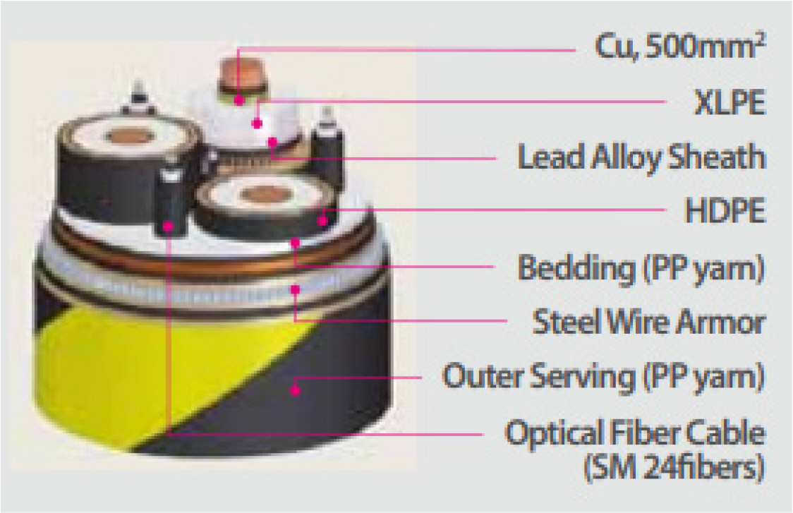
Components of subsea power cables
The mechanical properties of subsea power cables can be predicted based on experimental, theoretical, and numerical analysis using the finite element method (FEM). Lutchansky (1969) and Knapp (1979) proposed theoretical models for analyzing the stiffness and axial stress distribution of armor wires. In their research, bending, axial tensile, and torsional stiffness tests of subsea power cables were performed to investigate the correlation between the proposed equations and experimental results. Based on the research, subsequent studies on the mechanical properties of a range of subsea cables such as subsea power cables, umbilicals, and submarine pipelines were conducted through physical experiments and improved equations for the theory. Vaz et al. (1998), Coser et al. (2016), Ekeberg and Dhaigude (2016), Komperød et al. (2017), and Delizisis et al. (2021) investigated mechanical properties such as tensile stiffness and bending stiffness through experiments with full-scale subsea cables. Furthermore, Witz and Tan (1992), Huang and Vassalos (1993), Kebadze (2000), Skeie et al. (2012), and Komperød (2017) conducted studies on the analysis of the mechanical properties of subsea cables and prediction of the stress distribution in armor wires using numerical models, i.e., theoretical formulas. However, there has been limited research for verifying the validity of the proposed equations. Similar to the cases of other fields of research, the advancement in computer performance and the development of commercial software over the past decades have had a substantial impact on the research capabilities for analyzing the mechanical properties of subsea power cables. For example, the following are software programs specialized for the mechanical analysis of pipes and cables with composite hierarchical structures, such as subsea power cables: CableCAD; Helica; UFLEX; and commercial software based on the FEM, such as ABAQUS, COMSOL, and ANSYS. Shaw (2011), Lu et al. (2017), Tjahjanto et al. (2017), and Chang and Chen (2019) investigated the behavior of subsea cables by performing 3D finite element analysis. In addition, they compared the results of the numerical analysis with theoretical formulas or experimental results. Although these studies have demonstrated the effectiveness of numerical analysis based on FEM, numerical simulations using FEM incurs high computational cost.
In this study, experimental and theoretical analyses were performed to predict the axial stiffness of subsea power cables. Axial stiffness is a measure of the resistance to deformation along the longitudinal direction under an applied tension. In the experimental analysis, a uniaxial tensile test was performed on a 6.5 m three-core AC inter-array subsea power cable specimen by using a 10 MN hydraulic testing system. In the theoretical analysis, the axial stiffness of the subsea power cable specimen was predicted based on the theoretical framework presented by Witz and Tan (1992). Furthermore, the predicted results were compared with the experimental results.
2. Experimental Analysis
In CIGRE Technical Brochure (TB) 623 (CIGRE, 2015), the mechanical properties of subsea power cables are defined in terms of torsion, tension, bending, compression, impact, fatigue, penetration, friction coefficient, etc. In addition, the experimental methods for analyzing each property are described in detail. In this study, a uniaxial tensile test was performed to analyze the mechanical properties of subsea power cables subjected to tensile loading (axial stiffness), with reference to CIGRE TB 623. Subsea power cables (e.g., umbilicals, wire ropes, and mooring ropes) are slender bodies that are affected substantially by tensile loading in the longitudinal direction. To experimentally analyze the slender body specimen, the testing system described below was designed and fabricated to continuously withstand large loadings and to have a large stroke range of the crosshead to secure the length of the specimen and conveniently mount the specimen on the testing system. The hydraulic testing system for subsea power cables used in this experimental study has the following specifications: a maximum load of 10 MN, permissible specimen length of 4–13 m, maximum displacement of 700 mm, and maximum speed of 600 mm/min. Fig. 2 presents a schematic diagram of the hydraulic testing system used in the experimental analysis.
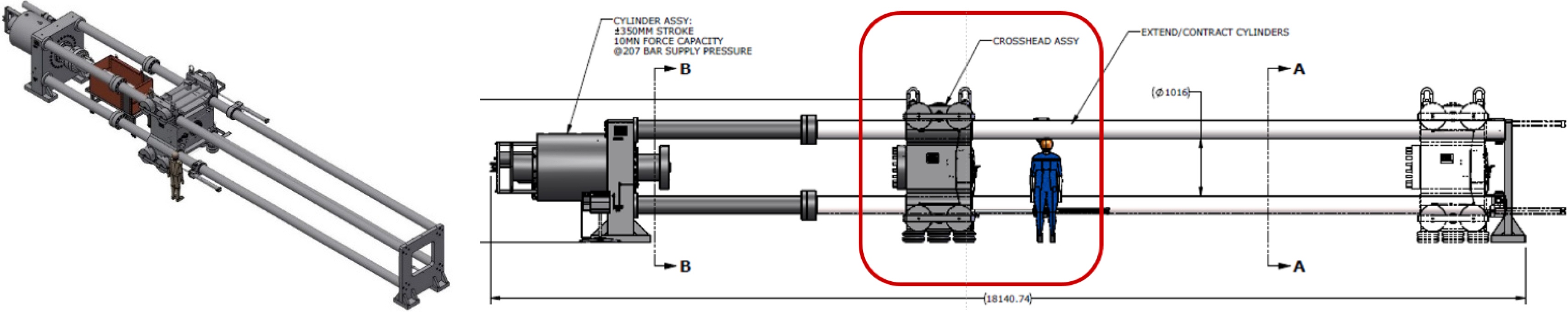
Schematic diagram of hydraulic testing system
A three-core AC inter-array subsea power cable was used in the experiment. Three-core AC inter-array subsea power cables are used for transmitting the power generated by offshore wind turbines to the offshore platform. In terms of axial stiffness tests, subsea power cables have two boundary conditions: fixed end–fixed end and fixed end–free end. In this experiment, only uniaxial tensile load was applied to the subsea power-cable specimen without rotation of the cross-section considering the fixed boundary conditions at both ends. An armor pot jig was specially designed and fabricated for modeling the complete fixed end condition at both ends of the cable. The armor pot jig was used for reproducing complete fixation by pouring silicone after connecting the fabricated metal frame to the end of the cable. The armor pot jig was connected to the hydraulic testing system at both ends. One end was connected to a hydraulic actuator to enable load control (See Fig. 3). The load and displacement data of the specimen were measured as functions of time and stored in the hydraulic actuator.
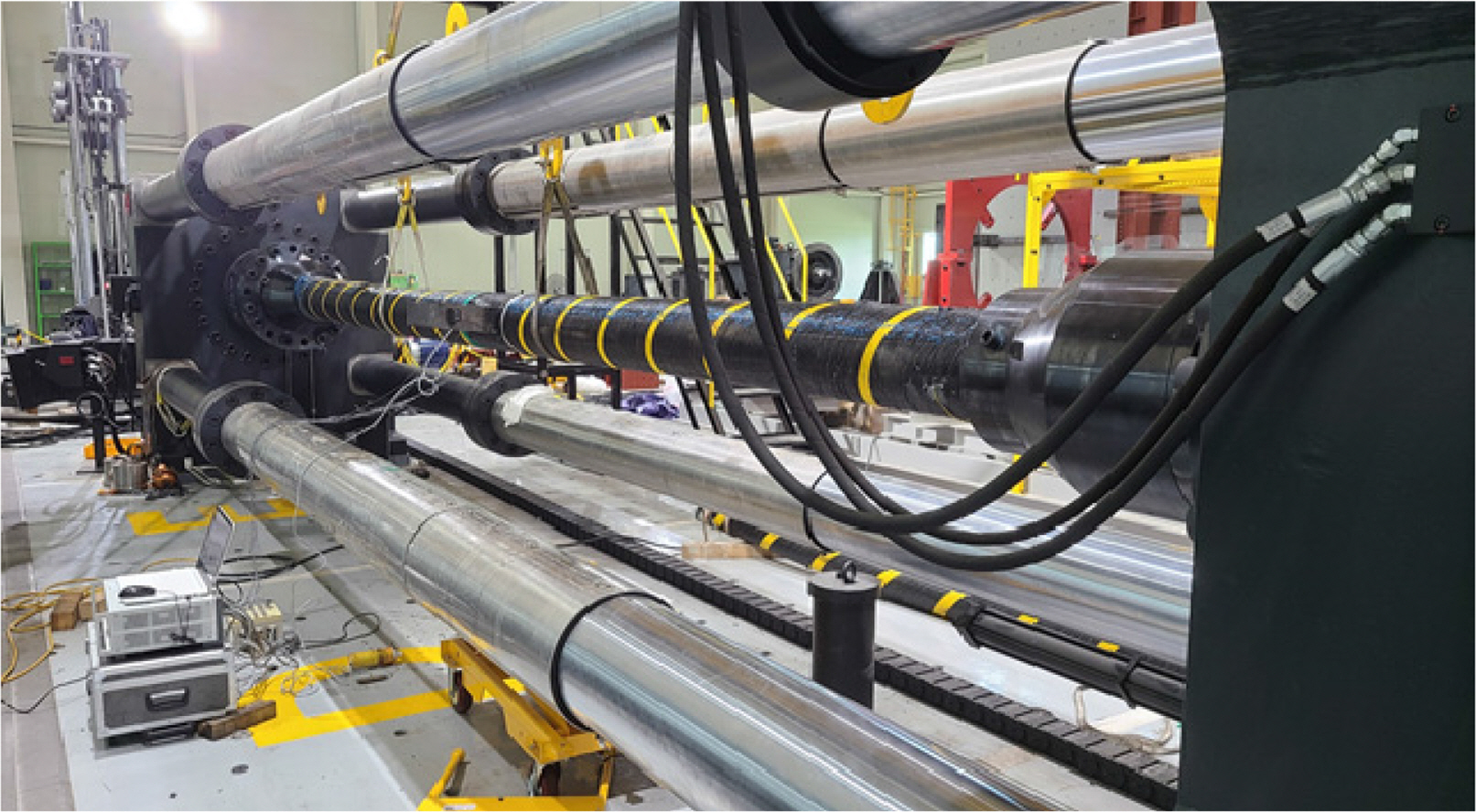
Uniaxial tensile test of subsea power cables
The length of the specimen was 6.5 m. An initial longitudinal displacement of 0.5 mm (a load of approximately 20 kN) was applied before the test to minimize the deflection caused by the self-weight. Three tests were performed on the same specimen. Fig. 4 presents the load–displacement curve of the specimen. As is evident from the figure, the subsea power-cable specimen shows a linear load–displacement curve in the three tests conducted. Table 1 outlines the axial stiffness values of the subsea power cables. The lowest axial stiffness value was obtained in the first test. This was because of the presence of significantly small gaps between each component layer during the fabrication of subsea power cables (Witz and Tan, 1992). The gap was minimized or removed after the first uniaxial tensile test. Consequently, the axial stiffness measured from the second and third loadings were constant.
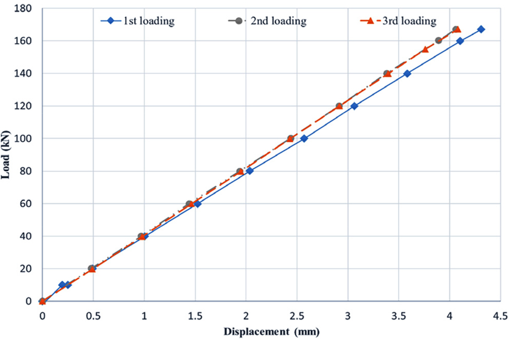
Experimental results: Load–displacement curves
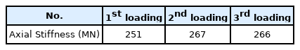
Experimental results: Axial stiffness
3. Theoretical Analysis
In this study, the theoretical models for predicting the mechanical properties of subsea power cables proposed by Witz and Tan (1992) were used. The equations are presented by dividing between cylindrical elements and helical elements. Consequently, these have advantage in terms of application to subsea power cables and to umbilicals and flexible pipes, which are hierarchical structures composed of cylindrical and helical elements. In addition, variations in the thickness and radius of each layer can be predicted because the interactions between component layers can be considered.
3.1 Theoretical Analysis of a Cylindrical Element
First, the equations for cylindrical elements proposed by Witz and Tan (1992) are based on the assumption of homogeneous materials. Fig. 5 shows the stress components of the cylindrical element.
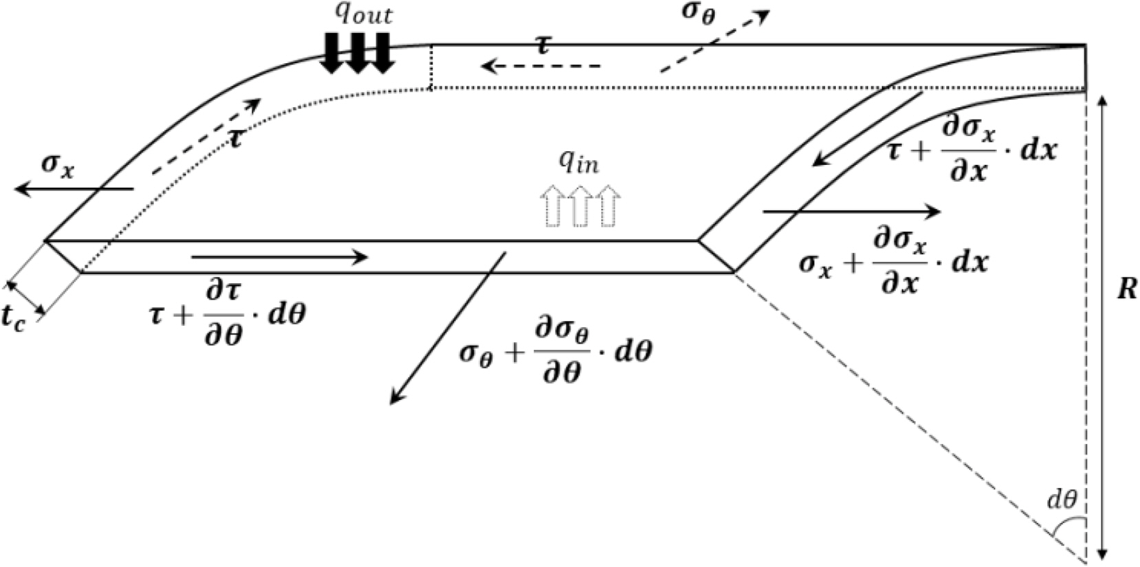
Cylindrical element stresses
The torsional load Mt; pressures on the inner and outer surfaces, respectively (qin, qout); and the stress components within the element when the cylindrical element is subjected to a constant axial load F are expressed as follows:
tc = thickness of the element
σx = axial stress
R= radius of the cylinder
σθ = circumferential stress
τ = shear stress
Assuming that uniform deformation occurs across the cylindrical element under a constant load, the strain components are expressed as follows:
∊x = strain in the longitudinal direction
∊θ = strain in the circumferential direction
∊r = strain in the radial direction
γ = shear strain in the plane of the element
L = length of the cylinder
ΔL = longitudinal deformation of the cylinder
ΔR = constriction of the cylinder
Δt = variation in the thickness of the cylinder
ϕ = twisting angle per unit length
In the equation for a cylindrical element, it is assumed that a constant out-of-plane stress is present owing to the pressures on the inner and outer surfaces. That is, the radial stress σr can be expressed as Eq. (8):
Assuming that an isotropic material is applied, the stress–strain relationship in the elastic domain is as follows:
E= Young’s modulus
v = Poisson’s ratio
G= Shear modulus
The stress components of the cylindrical element are derived as follows from Eqs. (9)–(12):
A relationship between the force acting within the cylindrical element and strain can be derived as follows by substituting Eqs. (1)–(8) into Eqs. (13)–(16):
3.2 Theoretical Analysis of Helical Elements
A distinct structural characteristic of subsea power cables is the presence of component layers of the helical elements. In the case of three-core cables, the core composed of the conductor of the subsea power cable, insulation material protecting the conductor, lead sheath, sheath, yarn, and armor wires have helical structures. The initial bending curvature and torsion of the helical elements according to the radius and pitch angle of the helical element layer are as follows:
K0 = initial bending curvature in the normal direction
K0′ = initial bending curvature in the binormal direction
Kt0 = initial twisting in the axial direction
R= initial helical radius of the strip
a = initial helical angle of the strip
Eqs. (24)–(26) show the final bending curvature of the helical elements when deformation occurs in the pitch angle of the helical component layer and helical elements owing to an arbitrary external force:
K1 = final bending curvature in the normal direction
K1′ = final bending curvature in the binormal direction
Kt1 = final twisting in the axial direction
∆R = constriction in helical radius
a1 = final helical angle of the strip
In the theoretical analysis of helical elements, the equation of elastic equilibrium presented by Love (2013) can be expressed as follows if the external force, shear force, and moment applied to the helical elements are assumed to be constant:
N′ = shear force in the binormal direction
B′ = bending moment in the binormal direction
T = axial force
X = distributed lateral force in the negative normal direction
H = torsional force
If the helical elements undergo deformation in the elastic domain, the bending moment and torsional load are proportional to the bending curvature and the variation in twisting, respectively:
EIh = binormal bending stiffness of the strip
GJ = torsional stiffness of the strip
The strain in the axial direction of the helical elements is expressed as Eq. (31):
∊a = axial strain of the strip
EA = axial tensile stiffness of the strip
According to the geometric relationship between the initial helical element and the helical elements after deformation, ∊a can be derived as a function of ∊x as follows:
a1 = helical angle of the stressed strip
Considering the geometric relationship again, a1 can be expressed as a function of ∆R, ∊x, and ϕ:
L = initial pitch length of the helical strip
The stress distribution in the normal direction of the helical element can be expressed in terms of the difference between the external and internal surface pressures: qout − qin =X/b. Here, b is the effective width of the helical element. From Eqs. (27) and (28), the pressure difference between the outer and inner surfaces of the helical element is rearranged and derived as Eq. (34):
The axial load generated in the entire layer of a helical element is equal to the sum of the axial loads of each helical element. Eq. (35) illustrates the axial load generated when n elements are present in the helical element layer.
3.3 Theoretical Analysis of Structural Characteristics of Subsea Power Cables Based on Composite Hierarchical Integration
In this section, we describe the method for theoretically analyzing a composite hierarchical structure considering the interaction of each layer when the cylindrical and helical layers are integrated in an arbitrary sequence. First, it is assumed that in the composite hierarchical structure, the respective cylindrical and helical layers have equal longitudinal strain (∊x) and twisting angle (ϕ) per unit length. The respective layers constituting the composite hierarchical structure interact with each other while undergoing different variations in radius or thickness under the action of an arbitrary external force. Furthermore, a governing equation is required to derive the expressions for the interactions of the respective layers. If a subsea power cable has m cylindrical layers out of the total n layers, we obtain the parameters of n variations in radius (∆Rn) and variations in thickness for m elements (∆tc,m). In conclusion, the theoretical model of Witz and Tan (1992) uses a nonlinear governing equation with ∆R as a single parameter. The process of deriving this governing equation is as follows:
The equation of equilibrium of the cylindrical element (Eq. (18)) and equation of equilibrium of the helical element (Eq. (34)) are expressed by the functions fc,j′ and fh,i, respectively. The subscript of the outer and inner surface pressure q indicates the number of the layer composing the subsea power cables. The number increases in the direction from the innermost layer to the outermost layer.
qint = internal pressure
qext = external pressure
In addition, the subscripts c and h denote cylindrical elements and helical elements, respectively. The cylindrical elements are identified by using a prime symbol in a subscript. The contact pressure q1⋯qn− 1 in Eq. (36) is offset by adding all the equations of equilibrium. This yields the following:
If the longitudinal deformation ∆L of the structure and the twisting angle ϕ are known, the function fh,k has a single parameter (∆Rk), and the function fc,i′ has two parameters (∆Ri′ and ∆ti ′). As is evident from Eq. (37), the thickness of the cylindrical element in the structure reduces, whereas that of the helical element does not. Owing to the interaction between adjacent helical element layers, the same variation in radius occurs (∆Ri− 1 = ∆Ri). Furthermore, the variation in thickness of the cylindrical element is equal to the difference in radius variation between the adjacent helical element layers (∆ti ′ = ∆Ri− 1 − ∆Ri′). Therefore, Eq. (37) can be expressed as a function of radius variation, ∆R1.
Here, we need to express the function F ′ in terms of a single parameter (∆R1). To achieve this, ∆t needs to be expressed as a function of ∆R1. From Eqs. (18) and (19), the internal contact pressure of the cylindrical element can be obtained as follows:
In addition, if the value of the initial internal pressure is known, from Eq. (36)qi ′ − 1 can be expressed as a combination of hierarchical helical elements as shown in Eq. (40):
The following is derived by substituting Eq. (39) into Eq. (40):
Eq. (38) (the governing equation) can be rearranged as follows:
The Newton–Raphson method was applied to solve the governing equation F (ΔR1) as described above.
3.4 Three-core AC Subsea Power Cable
The cross-section of subsea power cables can be divided into two parts in terms of mechanical strength: (1) the part that combines the conductor constituting the center of the cable, insulation wrapping the conductor, lead sheath, sheath, and shaped filler used to maintain the original shape of the cable, and (2) the layer of armor wires to increase the mechanical strength of the subsea power cables. Here, the mechanical strength of the centrally located insulation, lead sheath, sheath, and shaped filler may be considered negligible. This is because these have a significantly low elastic modulus or cross-sectional area ratio compared with the conductor and armor wires. Consequently, the cable is more affected by the deformation caused by the friction force between adjacent layers than the deformation caused by an external force acting on the subsea power cable. Therefore, in the theoretical analysis of this study, it was assumed that the mechanical strength of insulation, lead sheath, sheath, and shaped filler layers with low elastic moduli may be omitted. Rather, a simplified core combining the conductor, insulation, lead sheath, and sheath was assumed and applied to the theoretical analysis (See Fig. 6). The values of the physical properties of yarn and armor wires required for theoretical analysis were obtained from Tjahjanto et al. (2017). In addition, the average elastic modulus of 36,500 MPa and Poisson’s ratio of 0.4 were applied for the simplified core considering the elastic modulus of each layer and ratio of the cross-sectional area.
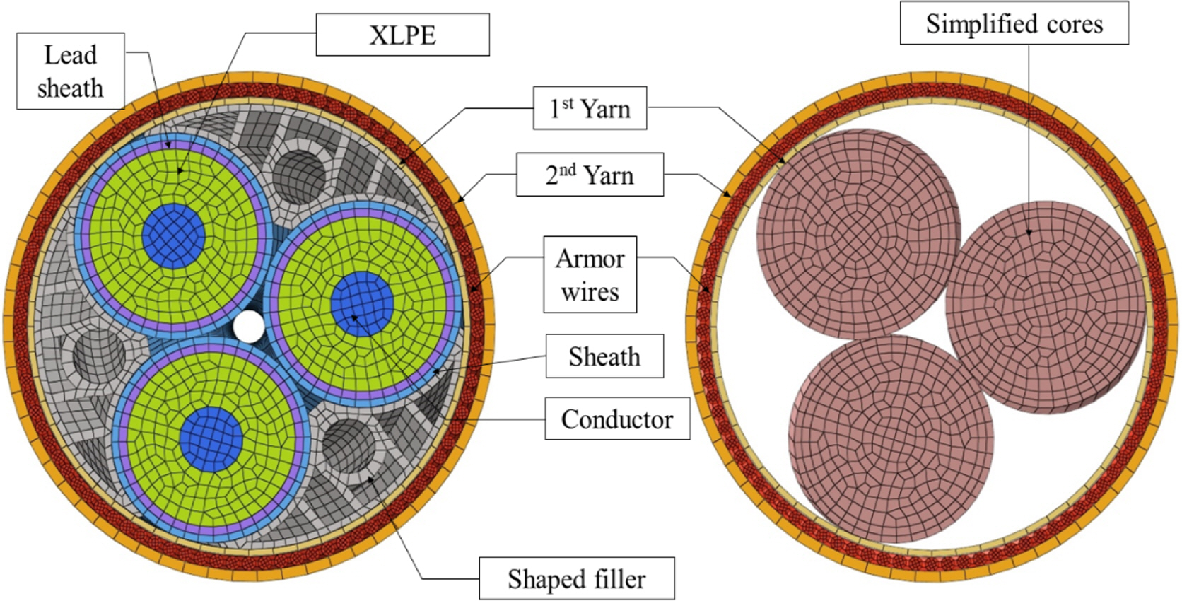
Cross-section of subsea power cable (left) and the simplified cross-section for theoretical analysis (right)
Accordingly, the subsea power cables used in the theoretical analysis were simplified to a composite hierarchical structure with four layers of helical elements (simplified core, first yarn, armor wires, and second yarn). Because all the components were helical elements, the thickness variation of each layer is not considered in the analysis. The thicknesses of the simplified core (1 core), first yarn, armor wires, and second yarn were 55, 2.2, 4.8, and 4.4 mm, respectively.
The values of the parameters required for the theoretical analysis are summarized in Table 2. In subsea power cables, there is no internal pressure as in the case of umbilicals or pipelines. Thus, the internal pressure (qint) is 0 N. The external pressure (qout) was also considered as 0 N because no external pressure was applied to the cable in the experiment.
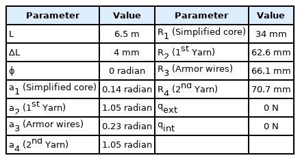
Parameters applied to theoretical analysis
Fig. 7 shows the load–displacement curve predicted by the theoretical analysis. Although the governing equation Eq. (42) is a non-linear function, the load–displacement (longitudinal deformation) curve is linear. The axial stiffness calculated from the theoretical analysis is 286 MN. The radius variation ∆R is 0.07 mm, which is insignificant (= 0.1% of the initial radius (approximately 75 mm)).
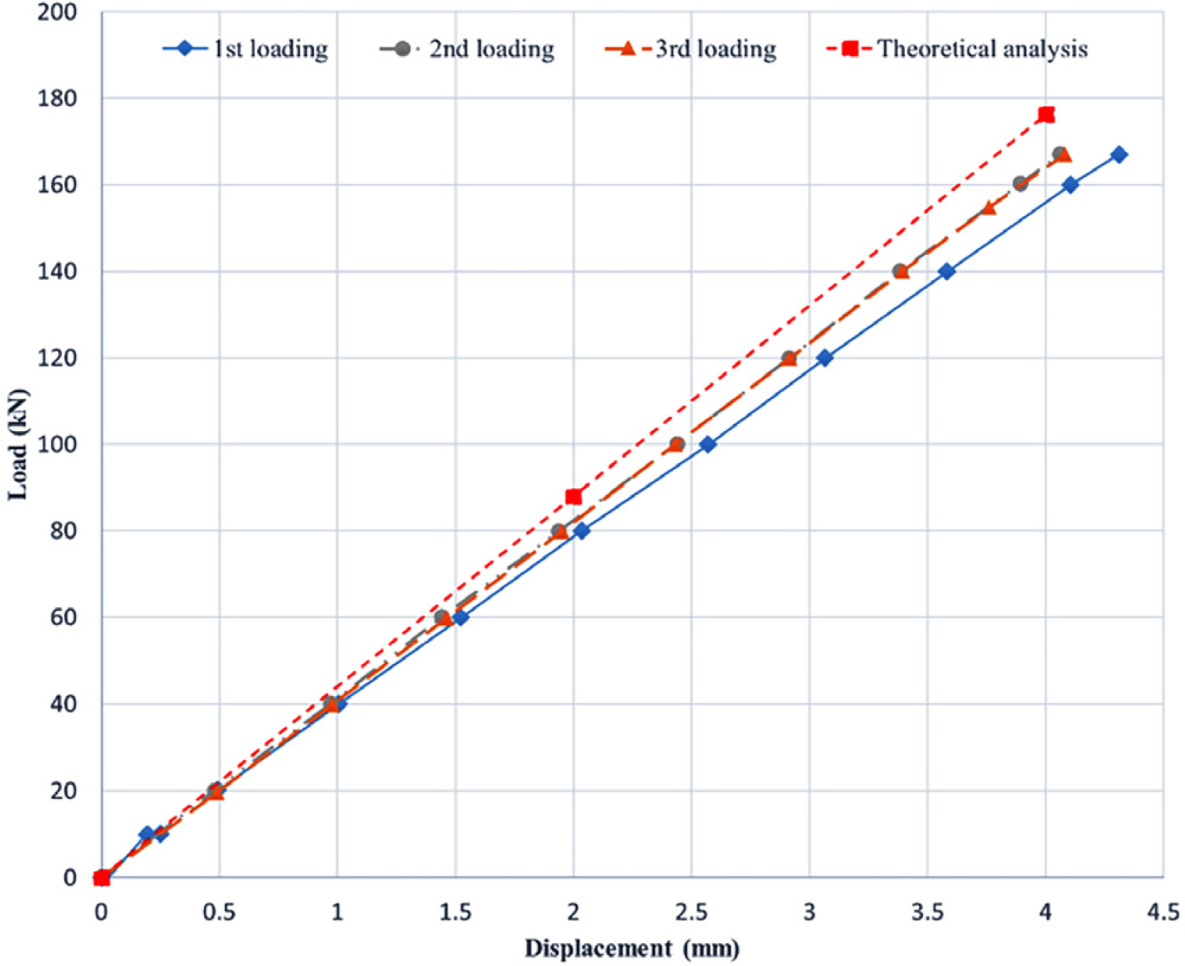
Theoretical result: Load–displacement curve and comparison with experimental results
4. Discussion and Conclusion
In this study, experimental and theoretical analyses were performed to evaluate the axial stiffness of three-core AC subsea power cables. For the experimental analysis, a 6.5 m inter-array subsea power cable specimen was fabricated to perform uniaxial tensile test. In addition, the axial stiffness of the specimen was predicted using the theoretical model presented by Witz and Tan (1992). Furthermore, the predicted results were compared with the experimental results. The theoretical model of Witz and Tan (1992) predicted higher axial stiffness (error rate of approximately 6.6%) compared with the experimental results. The following are considered to be the causes of the error between the experimental and theoretical analysis results. First, because the model does not consider the interaction between elements in each layer as in the theoretical assumptions, it does not consider the resistance generated by interference or friction between elements. Second, the theoretical model does not consider the plastic deformation of materials that may occur in the manufacturing process of subsea power cables. That is, the mechanical strength of the helical elements may be overestimated because it is assumed that the helical element layer does not have a normal-direction curvature during production. In manufacturing, plastic deformation of the material may occur when the pitch angle of the helical elements is excessive or the radius of the helical element layer is significantly small. This, in turn, reduces the mechanical strength of the entire cable. Third, errors may be caused by oversimplification of the material properties (modulus of elasticity) and mechanical properties (bending stiffness, torsional stiffness) of the central part of the subsea power cable, i.e., a three-core structure. Nevertheless, the theoretical model used in this study is convenient to apply and has a significantly high computation speed compared with numerical analysis based on FEM. Therefore, it is considered an efficient method for predicting the mechanical behavior of subsea power cables. However, further testing and validation by comparing the results of the FEM-based numerical analysis are required for quantitatively verifying the feasibility and effectiveness of the method.
Although the uniaxial tensile test in this study was performed under fixed boundary conditions at both ends, the real-world subsea power cables are exposed to fixed-end-free end boundary conditions in the process of manufacturing, shipping, transshipment, burial, and installation. It is known that the axial stiffness of subsea power cables decreases under the fixed end-free end boundary condition. In addition, a more in-depth analysis of the stress distribution within each component and the initial deformation occurring during manufacturing of the cable is required. To achieve this, it is necessary to further analyze the axial stiffness according to the boundary conditions and the stress distribution within the components, and to modify the theoretical models to reduce the above-mentioned errors.
Notes
No potential conflict of interest relevant to this article was reported.