According to Newton's second law, the governing equation of motion for a floating body can be expressed as Eq. (1). M_ij is the mass of a floating body, and ü_j is the acceleration of a floating body. The subscript i and j represent 6 degrees of freedom, 1 = surge, 2 = sway, 3 = heave, 4 = roll, 5 = pitch, and 6 = yaw. The restoring force Fires is calculated from the hydrostatic stiffness C_ij and the displacement of a floating body u_j as shown in Eq. (2). According to Cummin’s equation, the radiation force Firad is expressed as Eq. (3). It is important that t₁ should be long enough for the impulse response function K_ij to converge stably to zero. The wave damping coefficient B_ij(ω) obtained through frequency response analysis is used to calculate the impulse response function as shown in Eq. (5). The added mass m_ij(∞) can be calculated by Eq. (4). The wave excitation force Fiwv for the regular wave is defined as Eq. (6). F_i is the response amplitude operator (RAO) of the wave excitation force obtained by frequency response analysis, H is the wave height and ϕ is the wave phase. The mooring force Fimr due to the mooring line and the impact force Ficol due to the collision of the FOWT with the tanker are calculated in Abaqus.

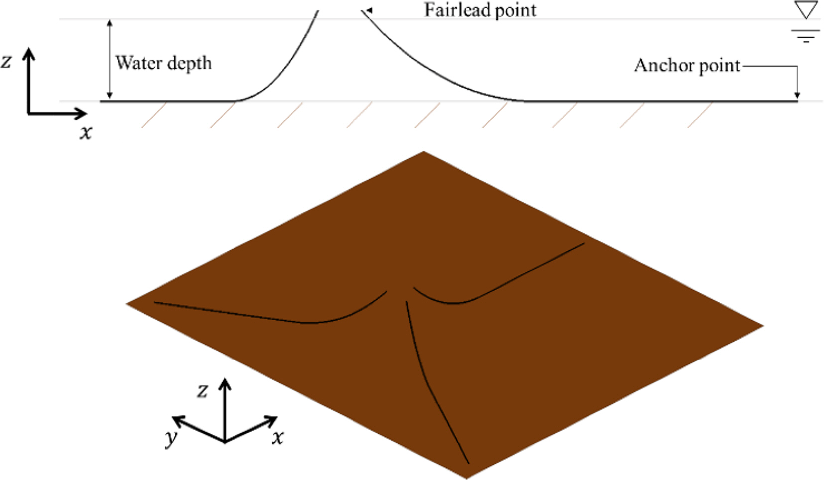
For modeling the mooring lines, the catenary equations presented in the studies of Masciola et al. (2013) and Jonkman (2007) were used, and are given by Eqs. (7)–(14). l and h denote the vertical and horizontal positions of the fairlead, respectively. H and V are the horizontal and vertical forces at the fairlead. EA, W, and L are the properties of the mooring line: axial stiffness, weight per unit length, and unstretched length. C_B is the friction coefficient between seabed and mooring line and L_B is the laid length on seabed. By calculating Eq. (10) and Eq. (11), the location along the line segment s is derived, which are used to model mooring lines.

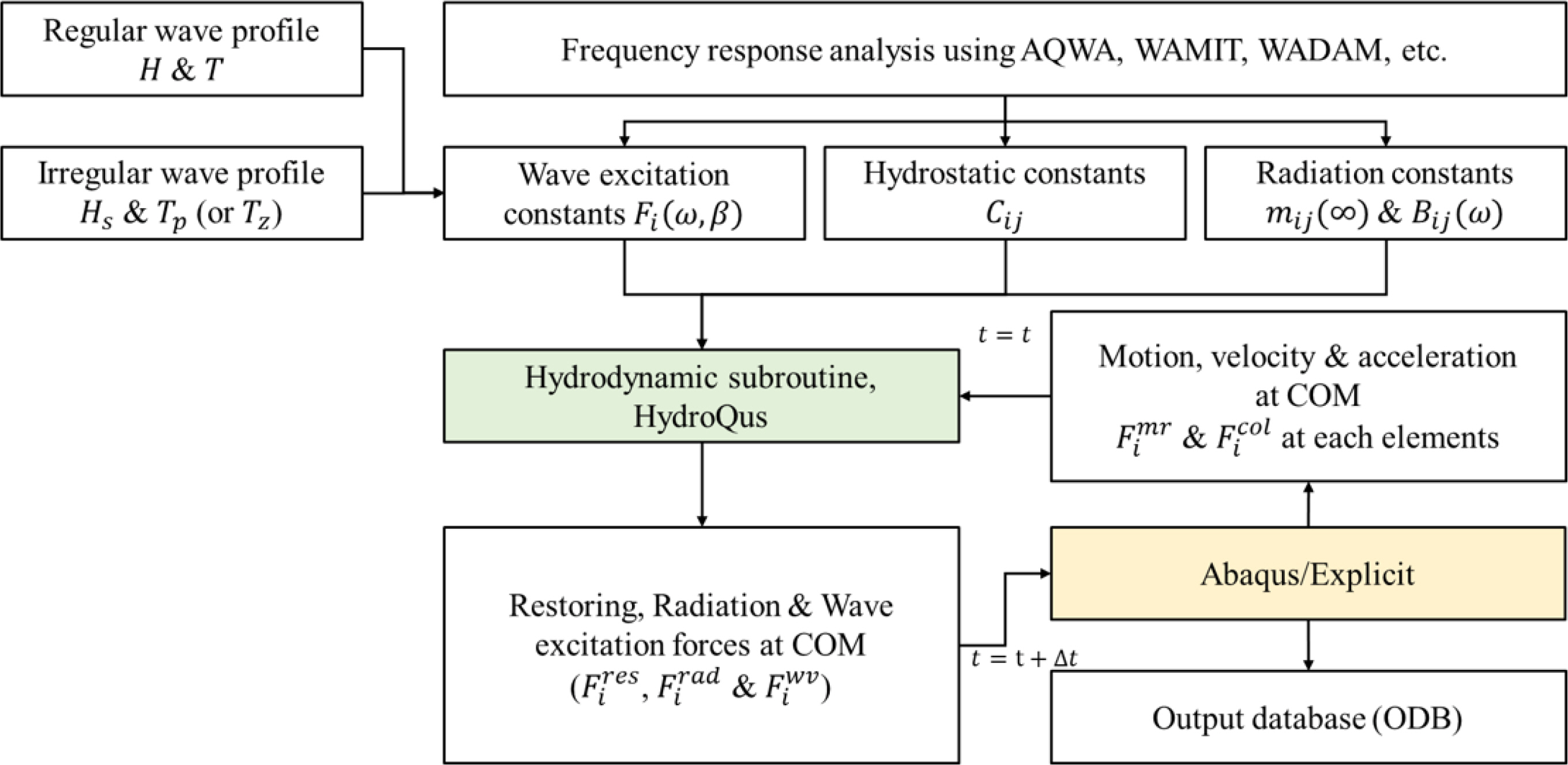
Abaqus is a commercial FEA code that includes a variety of material constitutive equations and a robust contact algorithm. However, Abaqus is not capable of generating hydrodynamic forces based on potential flow theory on its own. To solve this problem, the authors of this paper developed HydroQus, a hydrodynamic plug-in compatible with Abaqus/Explicit. HydroQus can generate linear or nonlinear restoring forces, radiation forces, and 1^st and 2^nd order wave excitation forces. The hydrodynamic coefficients used in the calculations must be obtained in advance from a frequency response analysis. For the wave excitation force calculation, the wave height H (or significant wave height H_s ) and wave period T (or peak period T_p) must be defined. HydroQus calculates the hydrodynamic forces using the displacement, velocity, and acceleration at the center of mass (CoM) of the FOWT at t= t₁ (current time) in Abaqus and gives them to Abaqus/Explicit. Abaqus solves the equations of motion for the FOWT and the ship, respectively, using the hydrodynamic forces. During this process, Abaqus is responsible for generating the drag-based mooring tension forces and collision forces. The displacements, velocities, and accelerations at the CoM obtained by solving the equations of motion are fed back to HydroQus and used to generate the hydrodynamic forces at t= t₂ (next time). This procedure is summarized in Fig. 1.

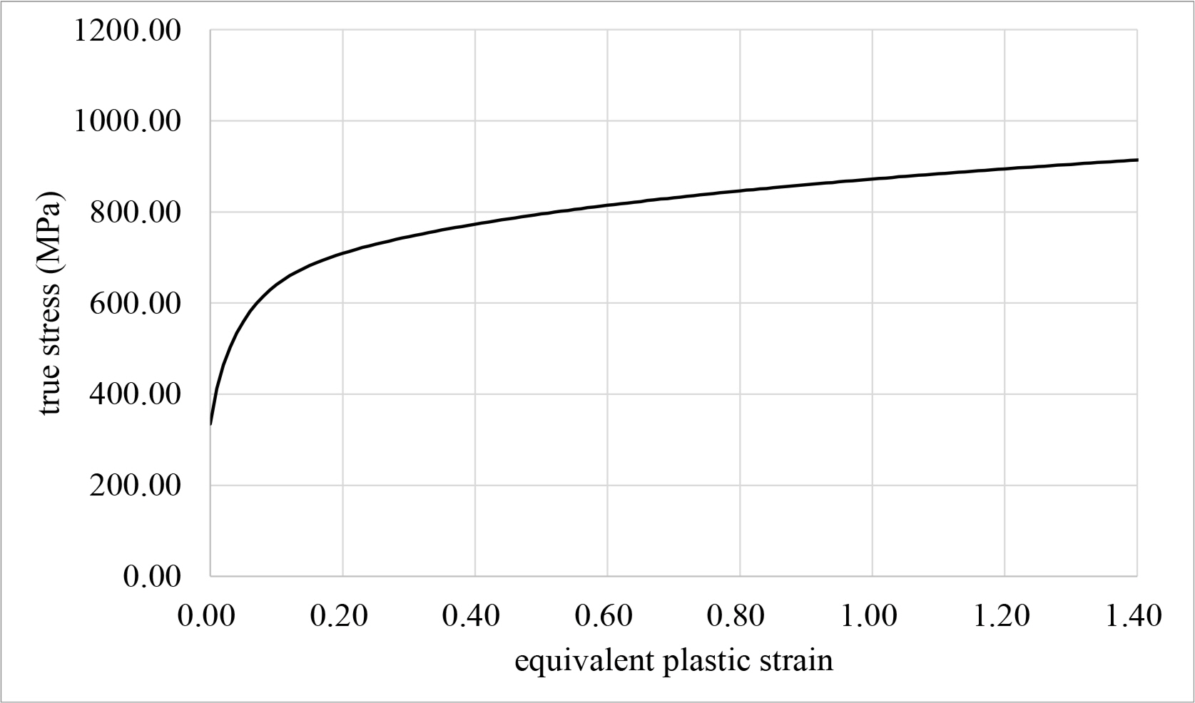
To accurately represent the hardening behavior after onset of necking, the combined Swift-Voce hardening model proposed by Sung et al. (2010) is applied in this study. The Swift-Voce hardening law is given by Eq. (15), where α is the weighting factor between Swift law and Voce law. The Swift law and Voce law are given by Eq. (16) and Eq. (17), respectively. Cerik and Choung (2020) derived A, ∊₀, n, k₀, Q, and β through tensile tests and numerical analyses.

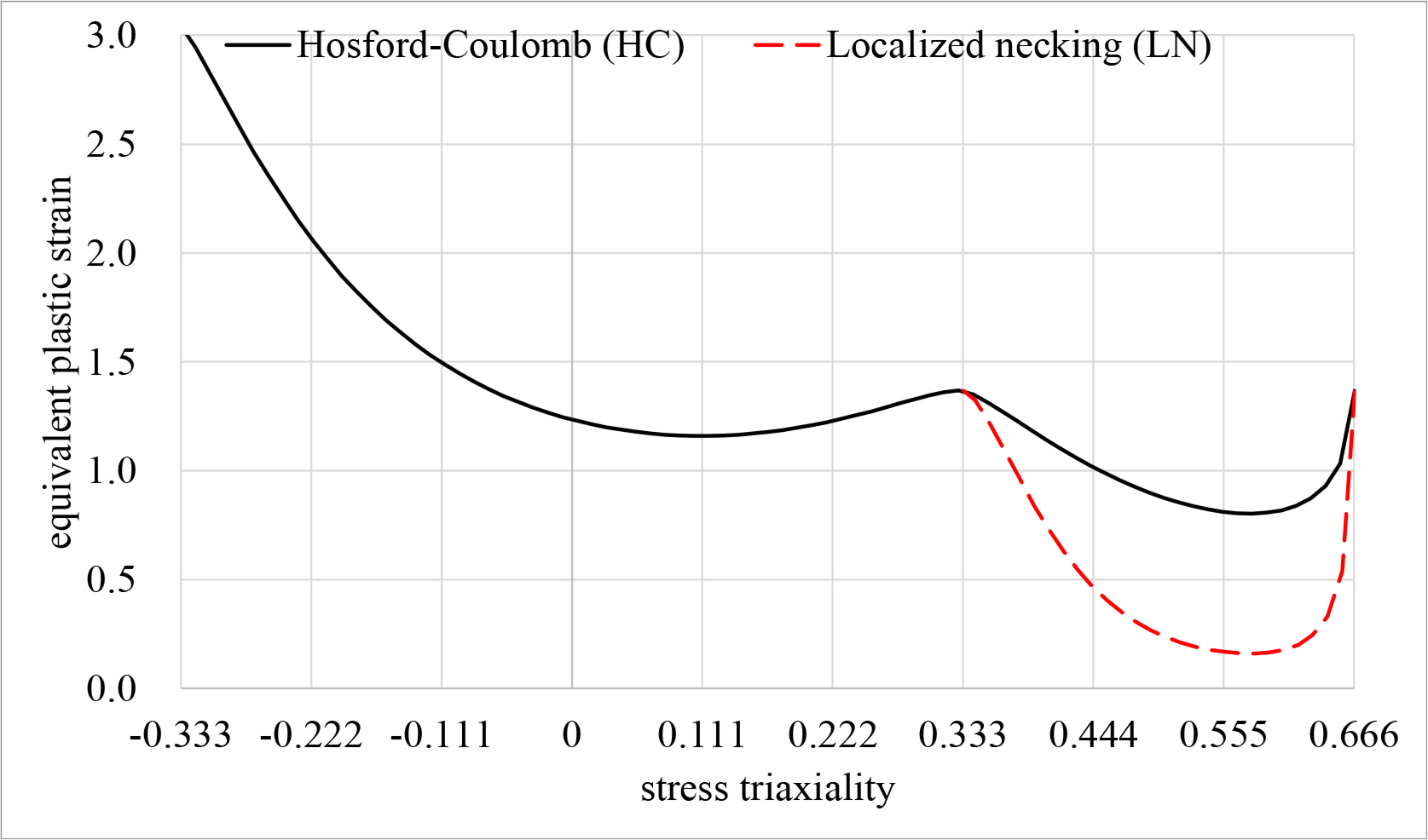
The fracture strain in the HC model proposed by Mohr and Marcadet (2015) is given by Eq. (18). Where η is the stress triaxiality and θ̄ is the Lode angle. From Eq. (18) and Eq. (19)a is the load angle sensitivity, b is the fracture strain modulus, c is the stress triaxiality sensitivity, and n_f is the transformation exponent. The load angle parameter functions f₁, f₂ and f₃ are calculated through Eqs. (20)–(22). To consider the stress path effect, the damage indicator D in Eq. (23) is introduced. It is assumed that fracture initiates when the damage indicator reaches 1.0.

The LN fracture strain model proposed by Pack and Mohr (2017) is given by Eq. (24). Where d is the Hosford exponent and p_f is the transformation exponent. Stress triaxiality functions g₁ and g₂ are calculated using Eq. (25) and Eq. (26). A necking indicator N is introduced to consider the stress path effect (see Eq. (27)). Fracture is considered to occur when N reaches 1.0.

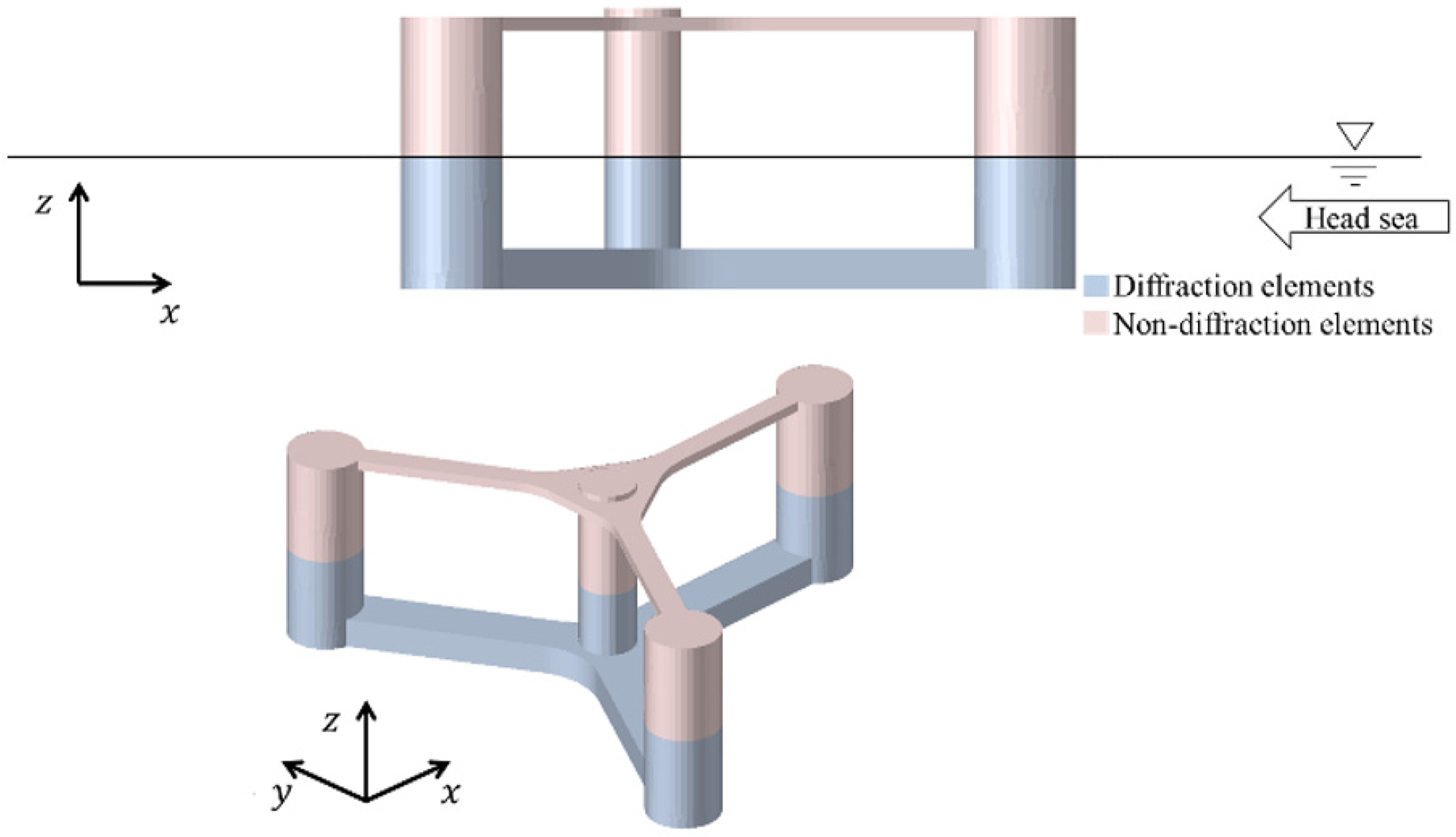
Fig. 2 is the model of FOWT used for the frequency response analysis. The frequency response analysis model consisted of approximately 5,500 diffraction elements and 4,500 non-diffraction elements. Tower and RNA were not included in the model, but were included in the mass information. Table 1 shows the mass information of the FOWT.

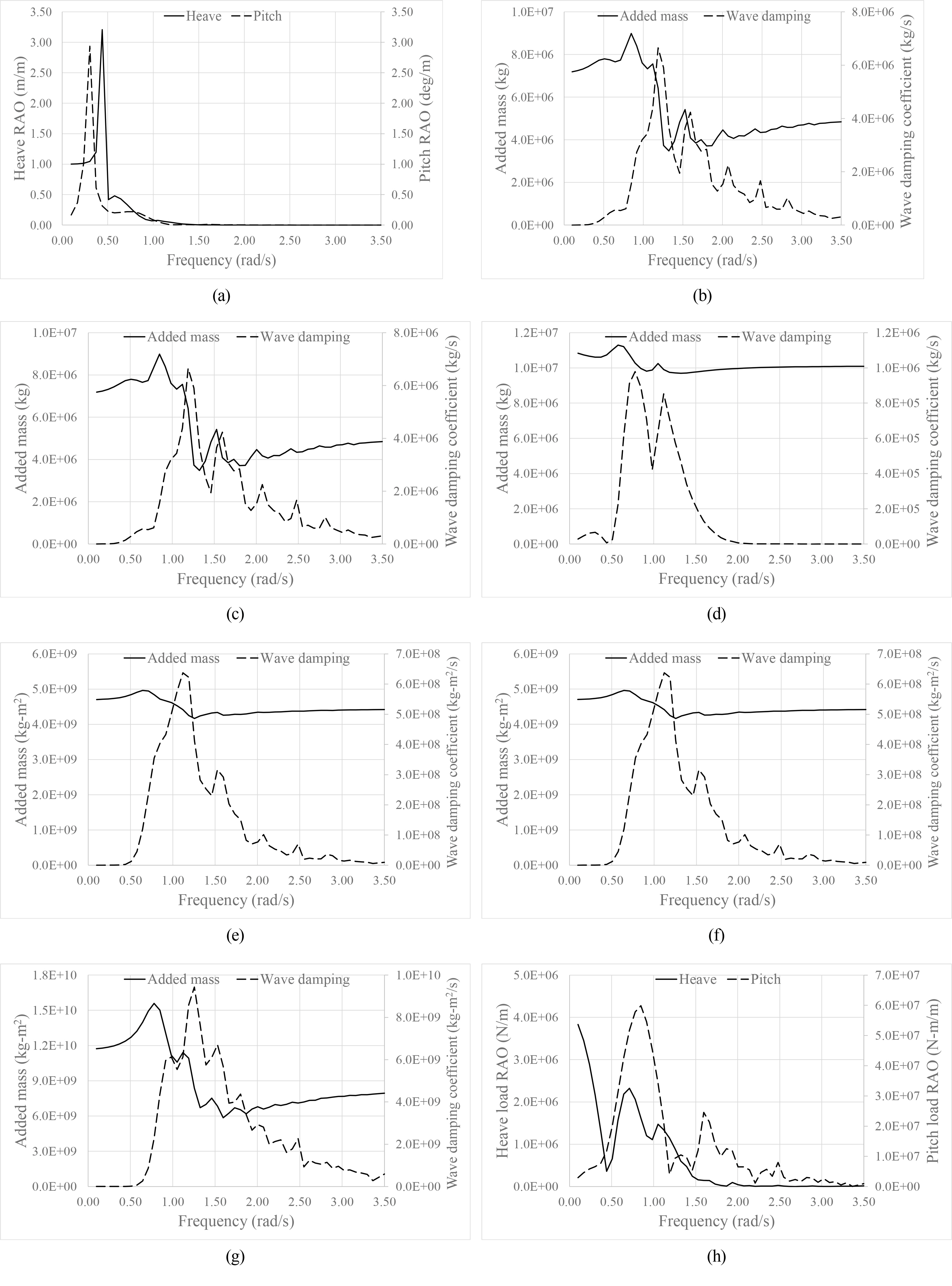
Frequency response analysis was performed using Aqwa (Ansys, 2022). The results of frequency response analysis in head sea condition are shown in Fig. 3 which includes the heave and pitch motion response amplitude operators (RAOs). The corresponding radiation coefficients for surge, sway, heave, roll, pitch and yaw motions are shown in Figs. 3(b)–3(g). It can be seen that the added masses nearly converged to a certain value as the frequency increased. The wave damping coefficients also nearly converged to zero as the frequency increased. Fig. 3(h) shows the 1^st order wave excitation force RAOs in the heave and pitch directions.

The tanker used in the collision simulations is shown in Fig. 4. In this study, the tanker was assumed to be a rigid body of R3D3 and R3D4 shell elements, while a MASS element, and a ROTARYI element were used to represent the mass. The main dimensions and masses of the ship are shown in Table 2.

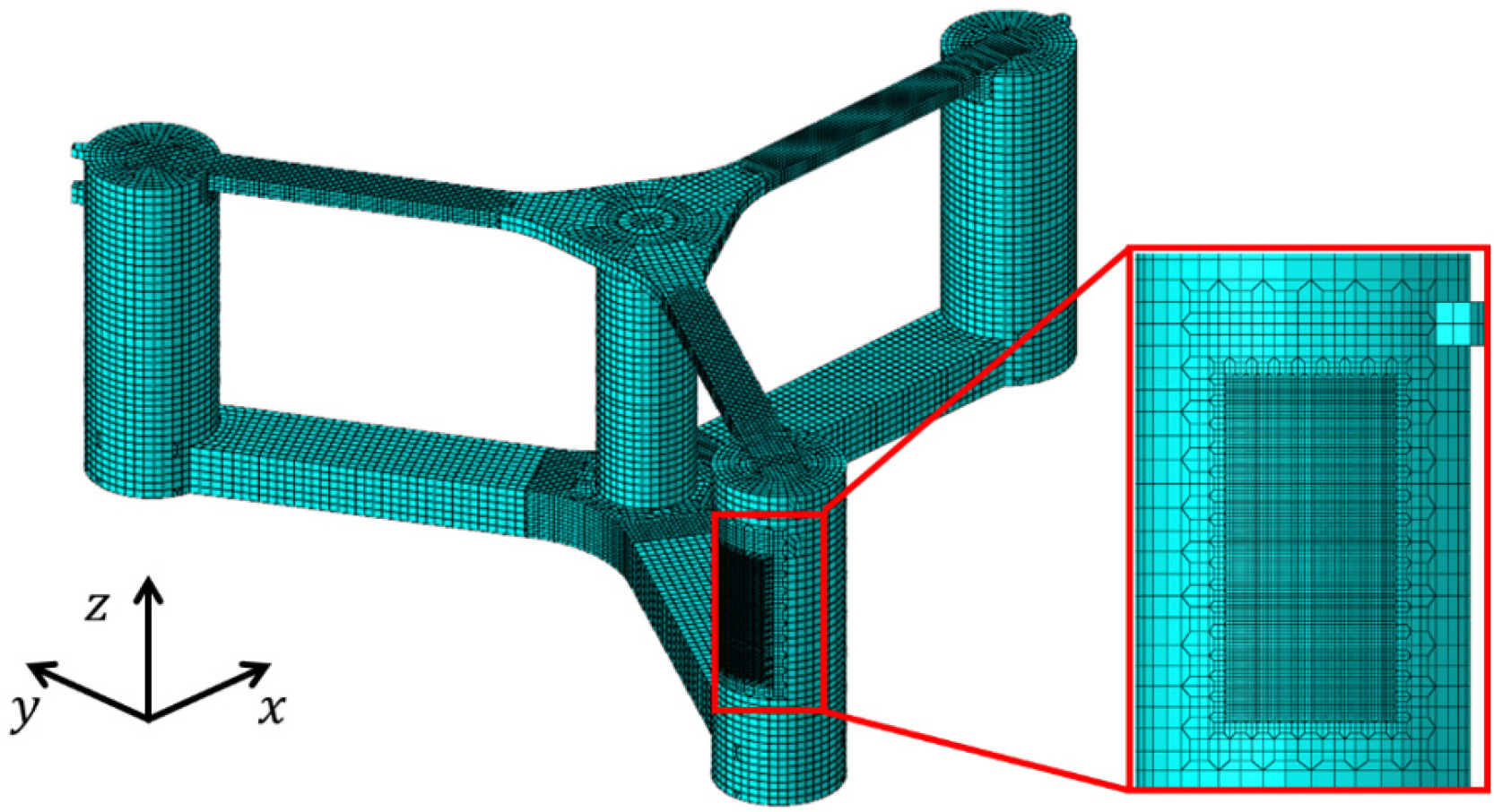
The FOWT was modeled with shell elements S3R and S4R. The element size was the longitudinal stiffener spacing, but the element size was reduced to 1/8 of the longitudinal stiffener spacing in the area where collisions were expected. The FEA model of the FOWT is summarized in Fig. 5 and Table 3.

The initial layout of the mooring lines was determined using the catenary equation. The mooring lines were modeled using beam element (B31) and joint element (UJOINT) connecting the beam elements to allow rotation. The seabed was modeled as a rigid element. The modeled seabed and mooring lines layout is shown in Fig. 6. Table 4 presents the modeling information of seabed and mooring line.

The DTU 10 MW wind turbine (Borg et al., 2015) released by the LIFES50+ project was used to model the tower and RNA (see Table 5). Fig. 7 shows the FEA model of the complete FOWT including mooring lines, floating body, tower, and RNA.

In this study, the floating body of the FOWT is made of AH36 steel for ship structures. In this study, the combined Swift-Voce hardening law was used to define the flow stress of this steel. The material constants of the combined Swift-Voce hardening law were determined based on the tensile test results by Park et al. (2020) (see Fig. 8). They also conducted a series of fracture tests. Their results were used in this study to obtain the fracture strain locus as shown in Fig. 9.

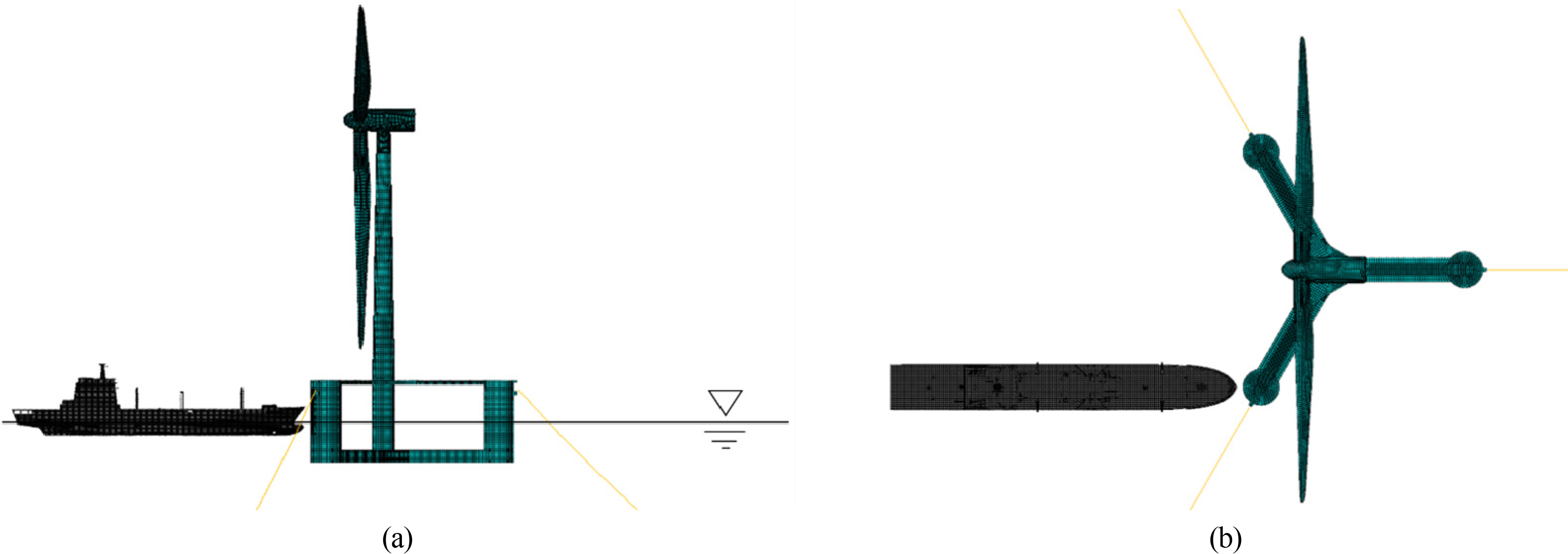
The objective of this study is unfolded into two. The first objective is to determine the impact of hydrodynamic forces on structural damage in a FOWT-tanker collision. Therefore, the cases were divided into those before and after considering hydrostatic restoring force and radiation force in the collision simulations. The second objective is to determine the impact of the fracture model on the structural damage assessment. For this purpose, the cases were divided into those with the HC-LN fracture model applied and those defined by a constant failure strain ∊_f. In this case, ∊_f was assumed to be 0.2, which has been the most widely used failure strain. Six cases were generated, which are summarized in Table 6. In all cases, the initial forward velocity of the tanker was assumed to be 5 knots (9.26 km/h). The collision analysis model is shown in Fig. 10.

The equivalent plastic strain is an important measure for determining the extent of damage. The equivalent plastic strain distribution just after the collision process is finished are shown in Fig. 11. Comparing the corresponding cases before and after considering hydrostatic force and hydrodynamic force (for example, comparing Case1-1, Case2-1 and Case3-1, or Case1-2, Case2-2, and Case3-2), there are no significant differences in the equivalent plastic strain distributions and maximum equivalent plastic strains. When comparing the constant failure strain model with the HC = LN model (e.g., Case1-1 and Case1-2), constant failure strain model shows similar damage extents as the HC-LN model, although the maximum equivalent plastic strains were developed up to 0.2 with the constant failure strain model.

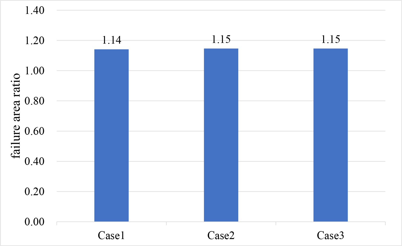
In this study, the damage extent is defined as the failed area of the side shell. The ratio of the damage extent with constant failure strain model divided by that with HC-LN model is shown in Fig. 12. In all cases, this ratio exceeds 1.0, which means that the constant failure strain model predicts larger damage extents than the HC-LN model.

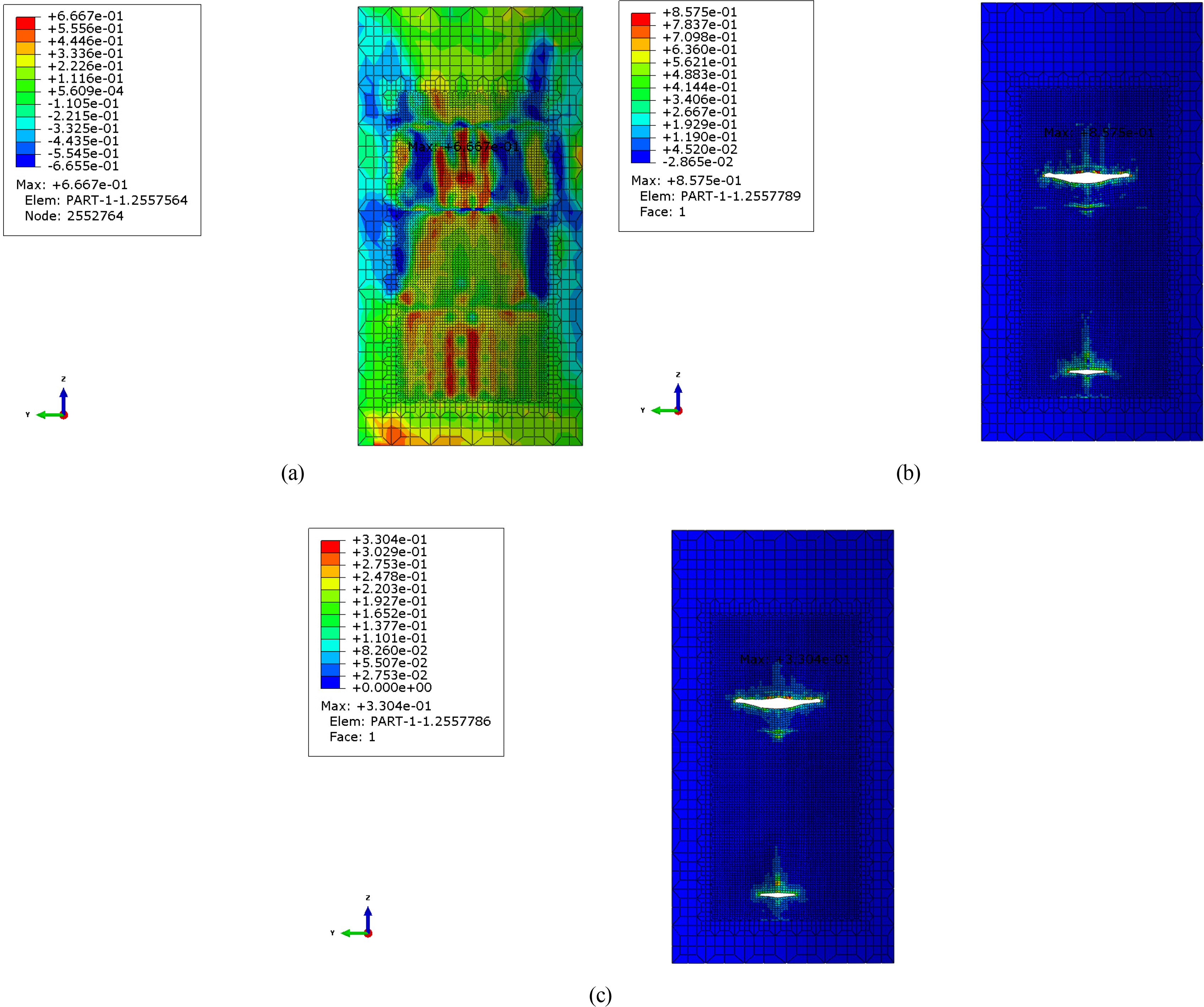
The stress triaxiality and damage indicators of Case3-2 were analyzed as an example. The stress triaxiality immediately after the collision occurred is shown in Fig. 13(a). It can be seen from Fig. 13(a) that the stress triaxiality in the collision area corresponds to the biaxial tension. A stress path at a fracture initiation location was formed with this stress triaxiality and the necking damage was accumulated. After the collision was completely terminated, the necking indicator and ductile fracture damage indicator are shown in Fig. 13(b)–(c), respectively. As expected, we can see that the LN necking damage indicator was developed much larger than the HC damage indicator.