Newton’s Method to Determine Fourier Coefficients and Wave Properties for Deep Water Waves
Article information

Abstract
Since Chappelear developed a Fourier approximation method, considerable research efforts have been made. On the other hand, Fourier approximations are unsuitable for deep water waves. The purpose of this study is to provide a Fourier approximation suitable even for deep water waves and a numerical method to determine the Fourier coefficients and the wave properties. In addition, the convergence of the solution was tested in terms of its order. This paper presents a velocity potential satisfying the Laplace equation and the bottom boundary condition (BBC) with a truncated Fourier series. Two wave profiles were derived by applying the potential to the kinematic free surface boundary condition (KFSBC) and the dynamic free surface boundary condition (DFSBC). A set of nonlinear equations was represented to determine the Fourier coefficients, which were derived so that the two profiles are identical at specified phases. The set of equations was solved using Newton’s method. This study proved that there is a limit to the series order, i.e., the maximum series order is N=12, and that there is a height limitation of this method which is slightly lower than the Michell theory. The reason why the other Fourier approximations are not suitable for deep water waves is discussed.
1. Introduction
The undulations on the water surface adopt inherently beautiful forms, such as the smooth regular features of progressive waves. On the other hand, despite the innate curiosity concerning water wave motion, it was only in the 19th century by Airy that efforts to provide a mathematical description of wave motion began in earnest (Henry, 2008). Since the early development of the theory describing the waves using the perturbation method by Stokes (1847), many nonlinear solutions were obtained, both analytically and numerically.
Based on the use of truncated Fourier expansions for flow field quantities, Chappelear (1961) and Dean (1965) developed a ‘Fourier approximation’ (Tao et al., 2007). By choosing the expansions to satisfy the Laplace equation and the BBC, the problem was reduced to solving a set of nonlinear equations for each of the Fourier coefficients, and the wave properties (Tao et al., 2007). As the set of nonlinear equations is derived from the finite series, the expansions were represented by truncated Fourier expansions, which is why they are coined as Fourier approximations. Considerable research (Chappelear, 1961; Dean, 1965; Chaplin, 1979; Rienecker and Fenton, 1981; Fenton, 1988) has been conducted on this approach.
The steam function theory was developed by Dean (1965). Dean (1965) proposed the use of the root mean square errors (RMSE) in the dynamic free surface boundary condition (DFSBC) and the kinematic free surface boundary condition (KFSBC) as an error evaluation criterion for wave theories. Dean (1965) also defined the Lagrangian function by introducing the linear summation of the two errors on the free surface with a Lagrange multiplier. Fourier coefficients were determined to minimize the Lagrangian function. The required order (N) of the stream function theory is determined by the wave steepness and shallow water parameter. For N = 1, the stream function theory reduces to the Airy wave theory. As the breaking wave height is approached, more terms are required to accurately represent the wave. Det Norske Veritas (DNV, 2010) described that stream function wave theory has an error of more than 1% in deep water waves whose height is over 90% of the breaking limit even though the required order is increased (See Figs. 3–4 in DNV (2010)). Chaplin (1979) applied the Schmidt orthogonalization process as an alternative to Dean’s method and obtained improved results (Tao et al., 2007).
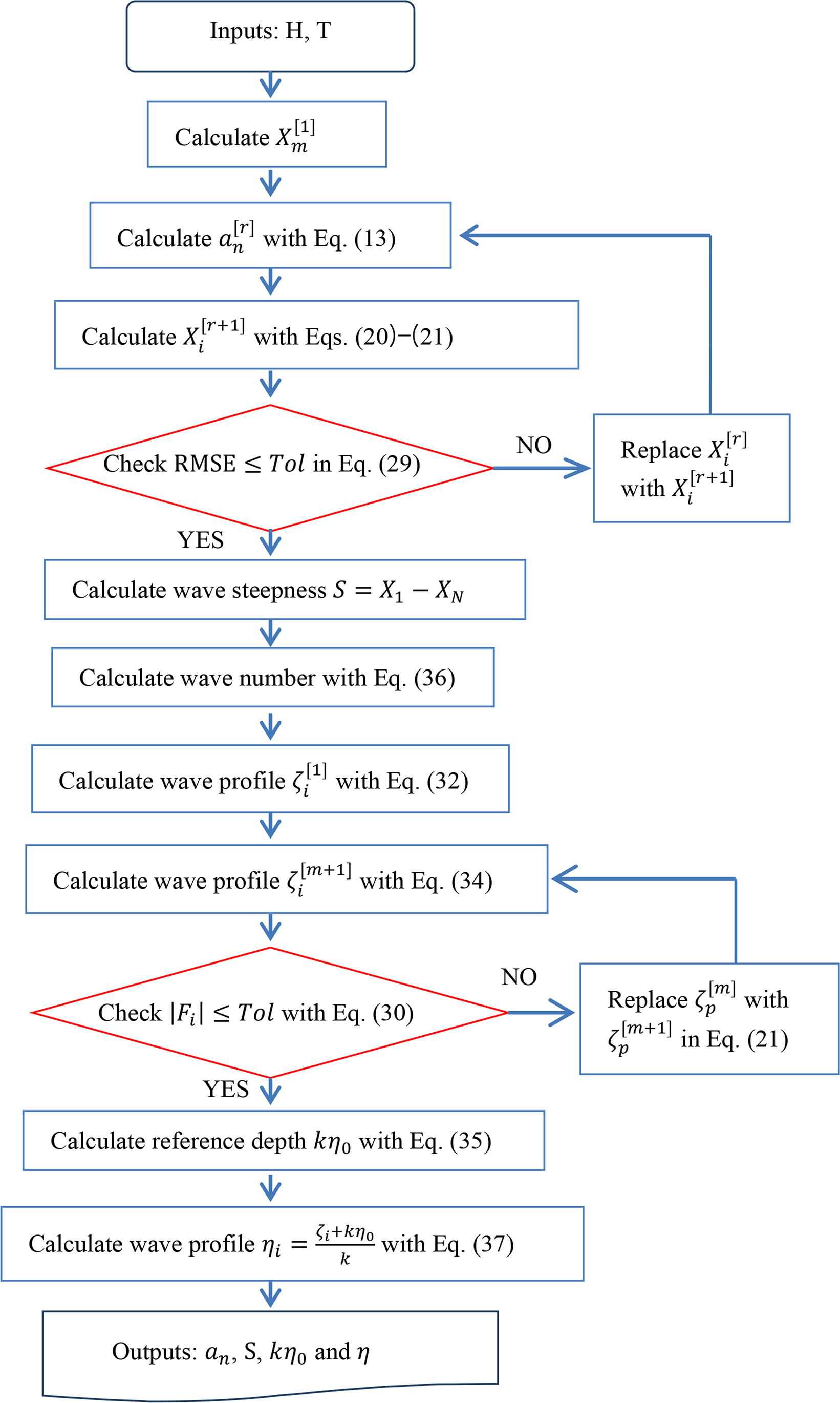
Flow chart for numerical analysis.
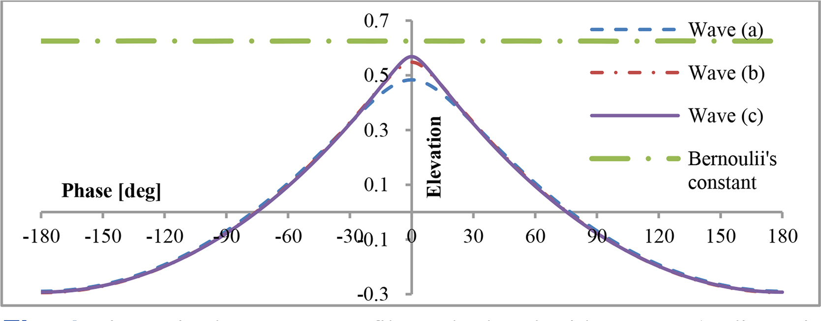
Dimensionless wave profiles calculated with N = 12 (ordinate is the dimensionless elevation from the still water line (SWL), kη)
Rienecker and Fenton (1981) also adopted the stream function introduced by Dean (1965). The unknown constants were calculated directly with Newton’s method in Rienecker and Fenton (1981). Therefore, the method required partial derivatives with regard to unknown constants, which complicated the numerical formulation of Newton’s method. Fenton (1988) obtained all the partial derivatives for simplification of this method numerically. Because the reference depth parameter is simultaneously determined with the Fourier coefficients, the required order should be increased to reduce the numerical error in the water depth condition. Newton’s method is unstable because the number of unknown coefficients increases when the required order increases. Therefore, the Newton method requires an initial solution closer to the exact solution. To solve it, in common with other versions of the Fourier approximation, it is sometimes necessary to solve a sequence of lower waves, extrapolating forward in height steps until the desired height is reached (Fenton, 1988). This problem can be avoided using the sequence of height steps (Fenton, 1990). As Rienecker and Fenton (1981) pointed out, several aspects of Fourier approximations beyond just the truncation of the series inhibited its widespread use (Tao et al., 2007). Neither of the above stream function approaches can be applied to waves in deep water because the stream function expansions contain hyperbolic functions (Fenton, 1988).
Shin (2016) reported that most numerical errors resulted from denominators in the stream function, the numerical integration of the water depth condition, and problems involved in Newton’s method. Shin (2016) solved the problems by separately calculating the water depth condition and introducing deep water velocity potential without denominators and a dimensionless coordinate system. The flow field was represented with a velocity potential to satisfy the Laplace equation and the bottom boundary condition (BBC). Two wave profiles were calculated by applying the velocity potential to the KFSBC and the DFSBC. The potential contains N+2 unknown constants, which are N Fourier coefficients, the wave steepness, and the reference depth parameter, while the stream function contains 2N+6 unknown constants (Rienecker and Fenton, 1981; Fenton, 1988). The wavelength and the reference depth parameter are not coupled to the Fourier coefficients because the dimensionless coordinate system was defined with the phase and the dimensionless elevation. Therefore, the wavelength and the reference depth parameter were determined independently. As a result, the required order was reduced in Shin (2016) and Shin (2021)
All the above-mentioned advantages resulted from the dimensionless coordinate system (Refer to Figs. 1 and 2). In addition to the advantages, there are some advantages to the coordinate system in Fig. 2. The independent variable is the relative horizontal position with regard to the wavelength in the moving coordinate system (Rienecker and Fenton, 1981; Fenton, 1988). The horizontal positions are also unknown values in Fenton’s method because the wavelength is an unknown constant, which makes the numerical procedure much more complicated. On the other hand, the independent variable is the phase in the range [0, π] in Shin (2016), which is a known value. In addition, partial derivatives with regard to the wavelength are unnecessary, unlike Fenton’s method (Rienecker and Fenton, 1981; Fenton, 1988). All the partial derivatives necessary can be calculated with tensor analysis, while they are calculated numerically in Fenton’s method. Therefore, there are no errors in the partial derivatives, unlike Fenton’s method. The numerical formulation of Newton’s method was also represented by tensor analysis.
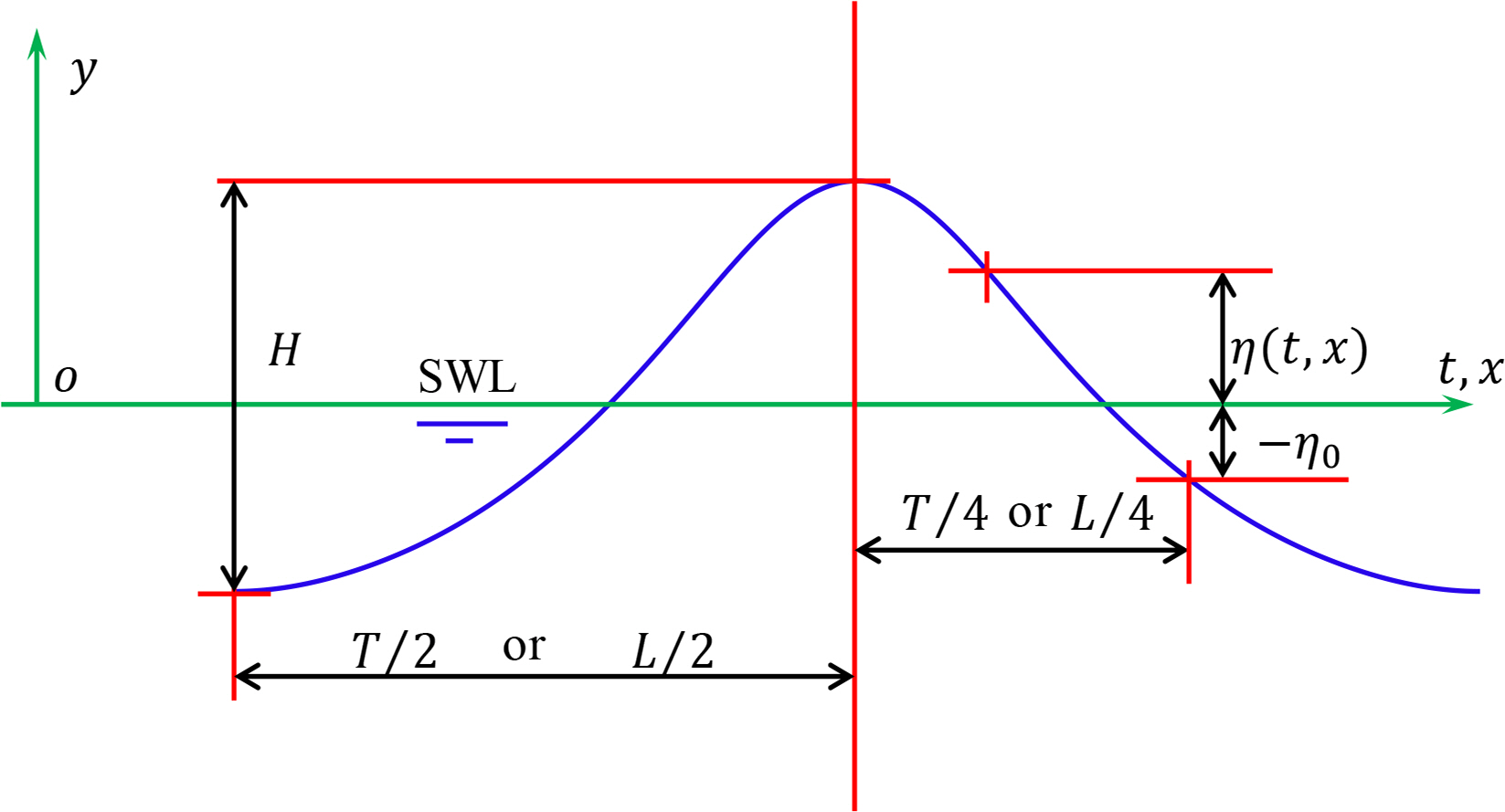
Conventional coordinate system for a progressive wave (H: wave height, T: wave period, L : wavelength, η(t, x): free surface elevation from the still water line (SWL)).
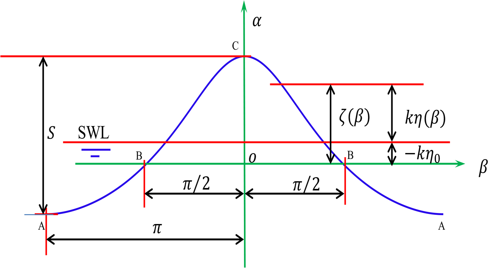
Dimensionless coordinate system for a progressive wave.
Some waves near the breaking limit were calculated for verification, and their errors were checked with Dean’s criteria. The deep water breaking limit was checked. According to the required order, the trend of numerical error was checked. There is a limit to the series order, i.e., N ≤ 12. This is why the other approximations are unsuitable for deep water waves.
2. Complete Solution
The complete solution was presented by Shin (2016), and the results are summarized in this chapter. Two coordinate systems were adopted to describe a progressive water wave. One is the conventional coordinate system (t, x, y) shown in Fig. 1. The origin is located on the still water line. The x-axis is in the direction of the wave propagation, the y-axis points upwards, and t is time. The fluid domain is bounded by the free surface y = η(t,x).
The other coordinate system (β, α) is the dimensionless stationary frame shown in Fig. 2. The origin is located at the point under the crest on the reference line, which is the horizontal line passing through two points at ηo = η (±90°) on the free surface. Therefore, the wave profile is a fixed, periodic, and even function in the system. The horizontal axis is the phase, β = kx − ωt, whose domain is −π ≤ β ≤ π, where k is the wave number defined by
The velocity potential in finite depth is represented in Shin (2019). The hyperbolic functions in the denominator are divergent as the water depth increases. Therefore, the potential is represented by the original deep water form without the hyperbolic functions.
The KFSBC is presented by an ordinary differential equation in the coordinate system. Solving the differential equation, the wave profile was calculated as follows (Refer to Appendix A):
The integral constant was determined by the definition of the reference line, i.e., ζ(±π/2) = 0. Eq. (6) contains only N coefficients, while Rienecker et al. (1981) contains N+5 unknown constants, which are N+1 coefficients, the wave number, celerity, volume rate, and Bernoulli’s constant. Compared to Rienecker et al. (1981), Eq. (6) is simple. Unknown constants are reduced dramatically by introducing the coordinate system in Fig. 2. Bernoulli’s equation is represented in the dimensionless coordinate system as follows:
Eq. (8) contains only N coefficients and wave steepness. In addition, Eq. (8) also satisfies that ζ(±π/2) = 0. Dimensionless wave height (steepness) is defined by
The steepness is determined by the wave height condition presented as follows:
For N → ∞, Eqs. (1)—(10) provide the complete solution to irrotational deep water waves. The solution contains N+2 unknown constants, i.e., the Fourier coefficient, an, wave steepness, S, and reference depth parameter, kη0.
This study aims to present a method to numerically determine the constants. N+2 equations are necessary to determine the unknown constants. The two profiles in Eqs. (6) and (8) should be identical for all phases. Hence, a set of N equations are obtained so that Eqs. (6) and (8) are equal at N phases. In addition, there are two equations, i.e., Eqs. (9) and (10). As a result, there are N+2 equations to determine the unknown constants.
An example for N = 1 and for N = 2 is presented in Appendix B and C, and Shin (2016) and Shin (2021) presented an example for N = 3. This method is further simplified and generalized by tensor analysis in the next chapter.
3. The Fourier Coefficients and the Steepness
A method to determine the Fourier coefficients and the steepness is presented for an arbitrary number of N.
In the other Fourier approximations (Rienecker and Fenton (1981), Fenton (1988)), the profile, η is directly calculated instead of ζ. Therefore, Eq. (9) must be simultaneously calculated with the coefficients. In this study, however, the profile η was calculated with ζ. Therefore, Eq. (9) was not coupled with the coefficients in this study and was calculated after they were determined. Hence, Eq. (9) is not considered in this chapter.
When the wave profile, ζ is prescribed in advance, it is possible to convert Eq. (6) to a set of linear equations to determine the coefficients. Because the wave profile is an even function, the phases βm for m = 1,2, ...,N are considered in the range, 0 ≤ βm ≤ π and βm ≠ π/2 because Eqs. (6) and (8) already satisfy that ζ(±π/2) = 0. β1 = 0 and βN = π. Letting Xm = ζ(βm), Eq. (6) is represented at the phase βm as follows:
The summation convention is considered in Eq. (11). The repeated subscript “n” is a dummy subscript. Kmn is a second-order tensor, an and Xm are vectors in N-dimensional space. The component of the tensor Kmn is presented as follows:
Using the inverse tensor Rmn of the tensor Kmn, the solution to Eq. (11) is determined easily as follows:
Using Eq. (8), the error vector Em in the DFSBC is defined as
The third-order tensor εijp is defined as follows:
A set of N nonlinear equations represented by Em = 0 for Xm are obtained by substituting Eq. (13) into Eq. (14). The set of equations is solved with Newton’ s method. A set of linear equations can be derived by denoting partial derivatives of a tensor using commas and indices as
Because
The superscript [r] with [ ] means the step of Newton’s method. All the steps are rth in all equations except Eq. (21) in this chapter. Therefore, for the simplification of equations, the superscript [r] was omitted in all the equations except Eq. (21). Differentiating Eq. (14) with respect to Xi, the partial derivative Em,i of the error vector is
Differentiating Eqs. (15)—(18) with respect to Xi, the components of the third-order tensors are
Because S = X1 — XN,
Differentiating Eq. (11) with respect to Xp, we have
Therefore, all the partial derivatives necessary were easily obtained without errors, unlike Fenton (1988).
Representing an individual component of a tensor as shown in Eqs. (12), (15)—(18), (23)—24), and (28), the summation convention was not considered. As a criterion of convergence, the Root Mean Square Error in the DFSBC proposed by Dean (1965) was adopted. Dividing the inner product of the error vector Em by N, the RMSE in the DFSBC (Dean, 1965) is defined as follows:
Newton’s method was rapidly convergent to the complete solutions (whose RMSE ≤ 10−13% within three steps) when the result of Shin (2021) was used as the first step solution. There are some differences in the above approach compared to Fenton’s method (Rienecker et al., 1981; Fenton, 1988).
All the partial derivatives with respect to wavelength are not required.
All equations can be formulated with tensor analysis.
Xi are merely parameters for calculating the coefficients and the steepness in this study. After determining the coefficients, Xt are no longer used. Hence, the wave elevation is denoted with Xi instead of ζi in Eqs. (11)—(28).
After determining the coefficients and the steepness, the wave profile and water depth condition were calculated separately, as presented in the next chapter.
4. Wave Profile and Reference Depth Parameter
The Fourier coefficients and the steepness were determined in advance. Therefore, the wave profile can be calculated with Eq. (6) as follows: Eq. (6) is represented as
Because F(β ζ) = 0, Eq. (31) provides a polynomial equation with regard to ζ. For q = 1, Eq. (31) provides a linear equation. Eq. (31) provides a quadratic equation for q = 2, and Eq. (31) provides a cubic equation for q = 3. The equations provide good approximations to the wave profile because |ζ| < 1 for all cases. For q=2, the following approximation is obtained:
The other root is a trivial solution because it does not satisfy that |ζ| < 1. The approximation is used as the first step in the Newton’s method defined as follows. The superscript [n] means the n’th step of Newton’s method (where n is a natural number), while the superscript (n) means the n’th order partial derivative with respect to ζ. The wave profile is calculated as follows by applying Newton’s method:
|F‘(β, ζ)| ≥ |F’(0, ζc)| for all waves and |F‘(0, ζc)| = 0 is the breaking condition proposed by Stokes (Chakrabarti, 1987). Therefore, Eq. (34) is valid for all waves except breaking waves. The Newton method rapidly converges to the complete solution. The wave elevations ζi = ζ (βi) were calculated using Eq. (33). Note that ζi stands for the free surface elevation at phase βi. The integral is numerically calculated by substituting the results in water depth conditions as follows:
Because ζ is an even function, β1 = 0, βi = (i − 1)π/M and βM+1 = π. Note that M is independent of N. When M is increased, Eq. (35) can be calculated more accurately rather than Rienecker et al. (1981) and Fenton (1988).
5. Numerical Analysis Procedure
Fig. 3 presents a flow chart of the procedure. The chart comprises two DO-loops because the Fourier coefficients and wave profile are independently calculated. The first step,
In this DO-loop, the Fourier coefficients and the steepness are determined. The wave number is calculated as follows:
The second DO-loop is used to calculate the free surface elevations at more phases than the phases considered in the first DO-loop. The elevations,
The water particle velocities were calculated by substituting the Fourier coefficients into Eqs. (2)–(3), and the accelerations were calculated by substituting the Fourier coefficients into Eqs. (4)–(5). The pressure field was calculated by substituting the Fourier coefficients into Eq. (7). The other wave profile was calculated by substituting the results into the right side of Eq. (8). The error in DFSBC can be checked by comparing the two profiles.
6. Results
The Fourier coefficients, an, the steepness, S, and the reference depth parameter, η0 are functions of one variable whose independent variable is the linear steepness, θ. Consequently, Shin (2019) numerically calculated some data for the coefficients, steepness, and reference depth parameters in the range, 0 < θ < 1. By curve fitting the data, the Fourier coefficients, steepness, and reference depth parameter are represented by Newton’s polynomials in Shin (2021), which give closed-form solutions. In this calculation, N = 3 was considered. The results satisfied the Laplace equation, the BBC, and the KFSBC. The RMSE in the DFSBC was less than 1% in the range, H/Lo ≤ 0.142 where Lo is the linear wavelength defined as follows:
Because θ = 2πH/Lo, H/Lo = 0.142 corresponds to θ = 0.892. As a result, Shin (2016, 2021) reported a good approximation whose error was less than 1% in the range, 0 ≤ θ ≤ 0.892. Although the error increases, Shin (2021) still applies to the waves in the range, 0.892 ≤ θ < 0.999. When θ > 0.999, wave profile by Shin (2021) does not converge. Each researcher has a different criterion regarding deep water breaking limitations. Chakarabarti (1987) proposes H/Lo = 0.142. According to Dean and Dalrymple, (1984), Michell theory is H/Lo = 0.17, which corresponds to H/L = 0.142. According to Stokes, the breaking criterion is u = c at the crest. In this study, the limitation was checked and the errors according to the required order were also checked. It is also discussed why the other Fourier approximations are unsuitable for deep water waves. For the verification, three waves with a period of 6 s are considered, which were tabulated in Table 1. The following series order was considered: N = 1; N = 3, 6, 10, 12, 13, and 35; M = 180. The RMSE in the DFSBC was calculated and tabulated in Tables 2 and 3. As the required order is increased, the error is decreased. When N ≥13, Newton’s method in Ch. 3 did not converge because eNζ is very large and aN is very small. As a result, this study is available for N ≤12.
Test waves with period T = 6 s

RMSE (%)

RMSE (%) as per Newton’s method step for N = 12
Eq. (35) was coupled with the other equations to calculate the Fourier coefficients, N = M and Eq. (35) is calculated with
The wave height to wavelength ratio was calculated, as listed in Table 4. The wavelengths were similar to the 5th-order Stokes wave. When θ > 1.028, this study does not converge. More precisely, Newton’s method does not converge because the wave profile at the crest is sharp when θ > 1.028. Therefore, θ = 1.028 is the limitation of this study, which corresponds H/L = 0.137 and is slightly less than 0.142 according to Dean et al., (1984).

Wave height to wavelength ratio, H/L.
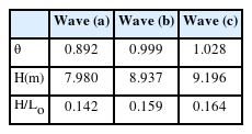
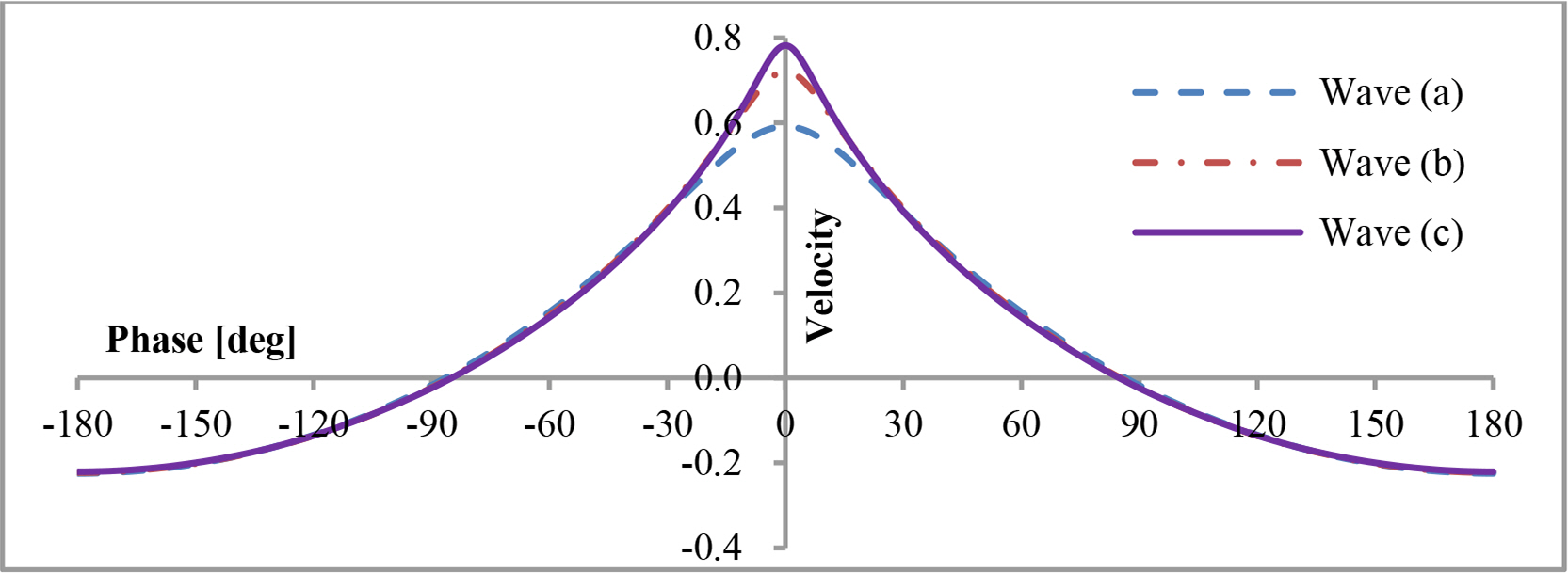
The convergent speed decreased when the required order increased. For θ ≤ 0.892, Shin (2021) is acceptable as the first step solution in Newton’s method. For θ > 0.892, the method reported by Shin (2021) is unsuitable for the first step solution because the Newton method does not converge. This problem can be avoided using the sequence of height steps. For waves in the range 0.892 < θ ≤ 0.999, the profile for θ = 0.892 is used as the first step solution, and for waves in the range 0.999 < θ ≤ 1.028, the profile for θ = 0.999 is used as the first step solution. The profiles are shown in Fig. 4; the horizontal velocities are shown in Fig. 5; the vertical velocities are shown in Fig. 6. The relative horizontal velocity at the crest is 0.782 for wave (c), which is less than Stokes’ criteria, 1. The Bernoulli’s constant in Fig. 4 is calculated for wave (c).
Relative horizontal velocities calculated with N = 12 (the ordinate is the dimensionless velocity, u/c)
Relative vertical velocities calculated with N = 12 (the ordinate is the dimensionless velocity, v/c)
7. Conclusions
This study aimed to provide a numerical method to calculate the Fourier coefficient, steepness, and reference depth parameter. The numerical procedure is much more simplified than Fenton’s method (Rienecker et al., 1981). The maj or simplifications are as follows:
Although the moving coordinate system by Dean was adopted in Fenton’s method, a dimensionless coordinated system was adopted in this study. As a result, all the partial derivatives with respect to wavelength are not required. Some parameters were eliminated.
All equations were formulated by tensor analysis. Therefore, numerical equations were much more simplified and had no errors.
In the other Fourier approximation, the required order was determined to reduce the error of the numerical integration in the water depth condition because it was solved simultaneously with the Fourier coefficients. On the other hand, the water depth condition was calculated independently. Therefore, the required order was reduced dramatically.
The error was reduced when the required order was increased. Nevertheless, there is a limit to the required order. This study is not applicable when N ≥ 13. Deep water breaking limitation was checked. This study is valid for waves in the range, 0 < θ ≤ 1.028. The limitation 1.028 correspond to H/L = 0.137, which is slightly lower than the Michell theory.
Notes
The authors declare that they have no conflict of interest.
References
Appendices
Solution to KFSBC
The KFSBC is presented in the conventional coordinate system as follows:
Because ζ = k(η − η0), we have
As ζ = ζ (β), then we have
And
Substituting Eqs. (A2) and (A4) into Eq. (A1), the KFSBC is presented in the dimensionless coordinate system as follows:
Substituting Eqs. (2) and (3) into Eq. (A5),
Because α = ζ on the free surface, then the water particle velocities are presented as follows:
Dividing Eq. (A6) by the celerity and multiplying the result by dβ
The above is presented as follows
Where the first term on the right-hand side of Eq. (A10) is presented as follows:
The second term on the right-hand side of Eq. (A10) is presented as follows:
The right-hand-side of Eq. (A10) is presented as follows:
Integrating the above equation,
Using the definition of the reference line (Refer to Fig. 2), we have
Solution lor N=1
For N = 1, the wave profile in Eq. (6) is represented as follows:
From Eq. (8), the other wave profile is represented as follows:
From Eq. (A16), crest height, i.e., the elevation at β = 0 is determined as follows:
Therefore, the Fourier coefficient is determined as follows:
From Eq. (A16), trough depth, i.e., the elevation at β = π is determined as follows:
By substituting Eq. (A19) into Eq. (A20) and substituting Eq. (10) into the result, ζt = −ζce−S. Substituting it into Eq. (10) allows the crest height to be determined as follows:
The trough depth is determined by substituting Eq. (A21) into ζt = −ζce−S:
The wave steepness is determined so that Eq. (A16) and Eq. (A17) meet at phase β = 0. Therefore the following equation can be used:
Eq. (A23) is the dispersion relation. For small amplitude, an approximation to Eq. (A23) is S = θ, which gives the linear dispersion relation ω2 = gk . Applying Newton’s method to Eq. (A23), the steepness was calculated as follows
Where S[1] = θ and
From Eq. (A23),
And differentiating Eq. (A26) with regard to S,
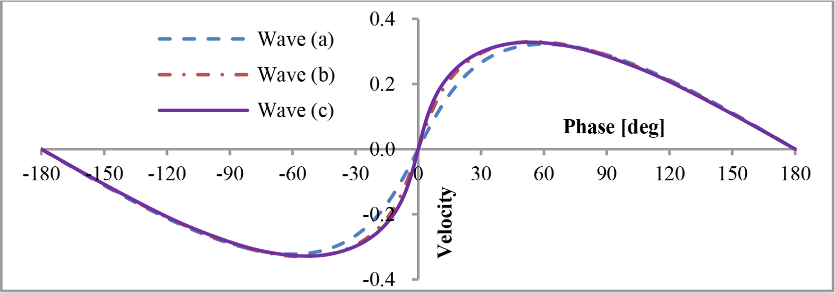
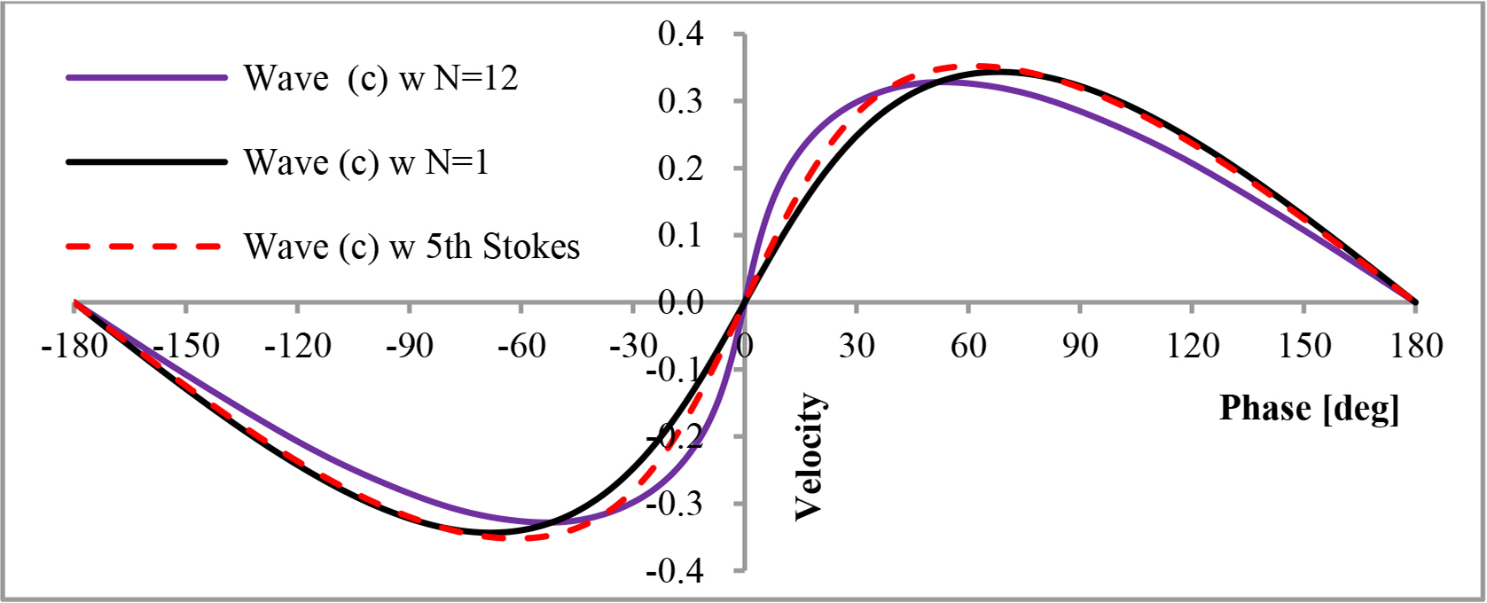
The wave profile is calculated with the method in Ch. 3, in which F(β, ζ) = −ζ + a1eζ cos β. This result has an error of less than 1.165% for waves in the range, H/Lo ≤ 0.142, which is less than the error of the 5th order Stokes’ wave theory. Wave (c) was calculated with N = 1, N= 12, and the 5th Stokes theory, and the results were compared in Figs. A1–A3. N = 1 gave similar results as the 5th Stokes theory. Comparing Fig. 4 and Fig. A1, the wave profiles calculated by N = 1, and the 5th Stokes theory was less sharp than those calculated by N = 12.
Dimensionless wave profiles calculated with N = 1, N = 12, and 5th Stokes theory (the ordinate is the dimensionless elevation from SWL, kη)

Relative horizontal velocities calculated with N = 1, N = 12, and 5th Stokes theory (the ordinate is the dimensionless velocity, u/c)
Relative vertical velocities calculated with N = 1, N = 12, and 5th Stokes theory (the ordinate is the dimensionless velocity, v/c)
Solution for N=2
For N=2, Eq. (6) is represented as follows:
Eq. (8) is represented as follows:
The coefficients are determined so that Eqs. (A28) and (A29) are equal to each other at phase β = 0 and β = ±π and to satisfy Eq. (10). Eq. (A28) is represented for X1 = ζ(0) as follows:
Eq. (A28) is represented for X2 = ζ(π) as follows:
Solving Eqs. (A30)—A31) for a1 and a2, the two coefficients are determined as follows:
The error of Eq. (A29) for X1 = ζ (π) is represented as follows:
The error of Eq. (A29) is represented for X2 = ζ (π) as follows:
Therefore, there are five equations, i.e., Eqs. (A32)—A35) and Eq. (10) to determine the unknown constants, a1, a2, X1, X2, and S. The set of equations was solved with Newton’s method presented in Ch. 3. The reference depth parameter and wave profile were determined using the method presented in Ch. 4.