


1. Introduction
It is essential to secure domestic front-end engineering and design (FEED) technology to ensure international competitiveness in the offshore plant industry, as well as to direct the deep-sea resource development industry and the new offshore plant industry market. To contribute to the technological development of the domestic shipbuilding offshore plant industry, it is imperative to build a large-scale ocean engineering basin to verify the performance of offshore plants and structures. The Korea Research Institute of Ships and Ocean Engineering (KRISO) developed the world’s largest deep-sea engineering water tank (100 m (length) × 50 m (breadth) × 15 m (depth)). It is equipped with complex equipment such as a wave maker, wind generator, current generator, depth control device, and towing carriage for the reproduction of the marine environment, including waves, wind, and current. The deep ocean engineering basin (DOEB) is used as a facility for design verification and performance/safety evaluation of existing oil and gas based on offshore structures and novel concepts for offshore plants.
The current generator is a major environment-reproducing facility and is useful for conducting motion and load characteristic tests on offshore structures. Offshore structures are significantly affected by the force of currents. The current force has an important influence on the structural characteristics, mooring lines, and risers. However, it is difficult to accurately predict the current force because the various fluidic interferences are rather strong.
Additionally, the current force has a significant influence on the motion characteristics of the structure and directly generates vortex-induced motions (VIM) in offshore structures (Finnigan et al, 2005; Lu et al, 2007). The current generator for the model test should consider the uniformity of the current, vertical current profile, and mutual interference between the waves and current. In particular, reproducing currents in deep-sea areas is an important issue, but it is quite difficult to consistently simulate currents for model tests. Because the flow is generated through a pump in the model test, relatively large flow irregularity may occur, and the uniformity may not be appropriate (Buchner and Wilde, 2008).
Because of these problems, the current flow uniformity of a large tank can be an important factor in a current load model test. However, it is difficult to find a study on a large tank current generator, which is not common. Therefore, it is necessary to consider how to circulate the tank water in a large tank to create a uniform flow. This study introduces a waterway shape design process to form uniform current flow and current velocity in a large tank and describes the design and installation process of an impeller system to rotate the water. Finally, after installation, the performance of the DOEB current generator was reviewed and compared with the design target factors.
2. Design of Current Generator in DOEB
2.1 Numerical Analysis for Design of Current Channel (Waterway) in DOEB
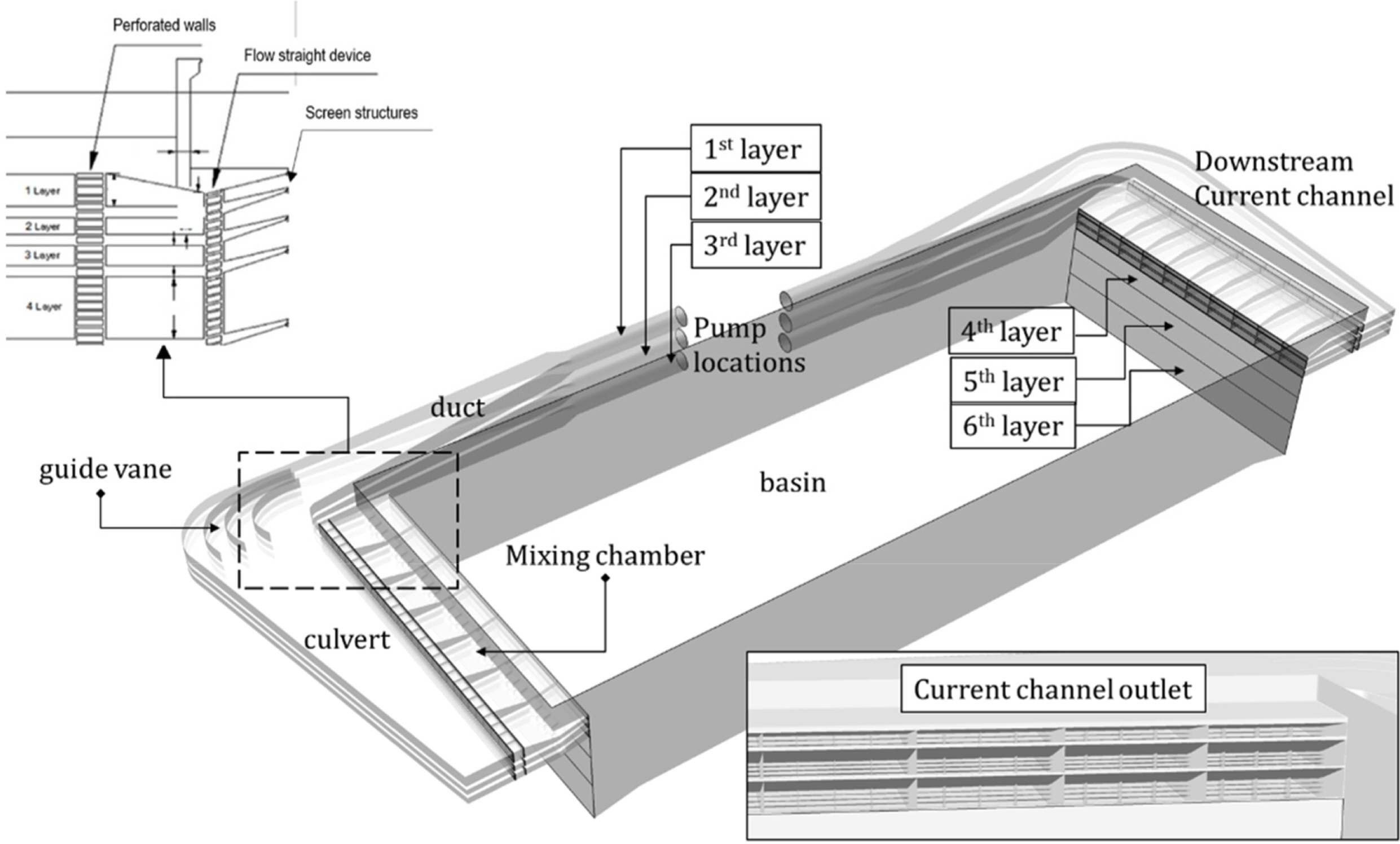
To implement a current generator that gyrates approximately 100,000 tons of water in the DOEB, the shape and specifications of the current channel and flow straightening devices for current uniformity were designed through numerical analyses. The main components and shape of the current channel of the DOEB across six stages of vertical waterway are shown in Fig. 1, which illustrates the culvert of the square guide pipe connected to a circular current pump pipe, guide vane located at the junction of the 90°-bend inside the culvert, mixing chamber, and current channel entrance. The mixing chamber is one of the important components in the current channel system for uniform current generation.
The water in the basin that is accelerated by the impeller of the current pump flows into the duct and culvert through the guide pipe and then exits into the basin through the mixing chamber, which has perforated walls and screens to generate a uniform current flow. The uniformity of the current flow in the test zone of the DOEB is very important for accurate offshore platform tests. To determine the shape and size of the current channel, the hydrodynamic performance of the current generation system was simulated through a computational fluid dynamics (CFD) approach. In this study, all simulations were carried out using the general-purpose software STAR-CCM+ (Siemens, 2018). The flow in the current channel was assumed to be turbulent and stationary.
The realizable k-ε turbulence model was employed for the turbulence closure of the Reynolds-averaged Navier-Stokes (RANS) equations. The SIMPLE (semi-implicit method for pressure linked equations) algorithm was used for the pressure-velocity coupling with the control of the overall solution. A second-order upwind scheme was used for the convection terms of the RANS equations, while a central difference scheme was applied to the diffusion terms.
To a certain extent, high flow velocities, velocity gradients, and turbulence intensities transferred by the pump decrease as the flow passes through the current channel system. However, relatively large-scale non-uniform flow structures can still be prominent, which makes it difficult to meet the required uniformity of the current flow in the basin. For this reason, the DOEB adopted perforated walls and screen structures that have some degree of solidity to make large-scale non-uniformities in the flow decay sufficiently and to control flow irregularities. The perforated walls are placed at the entrance of the mixing chambers and the exit of the tapered culvert section, while the screen structures are located at the entrance of the basin.
The present study used a screen model based on a wire mesh in the flow simulations to reproduce the solidity of the perforated walls and screen structures. The solidity of the wire mesh screen is easily calculated based on the diameter of wire and the size of mesh section (Lindgren and Johansson, 2002). This solidity effect can be modeled as an inertial resistance force term in the governing equations (Siemens, 2018) as follows:
where Pv is the viscous resistance, Pi is the inertial resistance, and V̄ is the mean velocity through a perforated wall with a given degree of solidity. The current study neglected the viscous term and calculated the inertial resistance by using a pressure loss formula as follows:
where ρ is the fluid density, Ko is the loss coefficient, Red is the Reynolds number based on the diameter of wire screen, and β is the solidity. f(Red) is a function of the pressure drop and has a converged value of 0.5 at Red > 100. More details of the numerical methodology can be found in a previous study (Park et al., 2014).
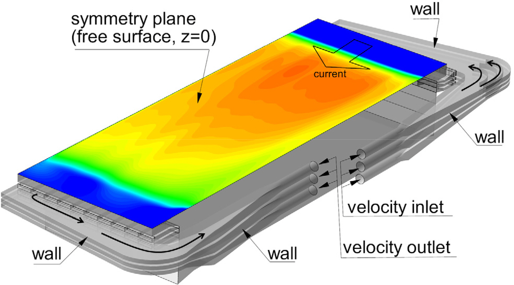
The computational domain was the DOEB itself. As shown in Fig. 2, the free surface in the DOEB was modeled as a symmetry plane without deformation. The inlet and outlet sections of the upper three current channel layers had the same velocity condition, which corresponds to the average velocity at the impeller plane generated by the pump at each layer. For the remaining lower three channel layers, constant inflow velocities were imposed at each channel exit to the basin. Wall boundary conditions were applied to all other surfaces of the DOEB.
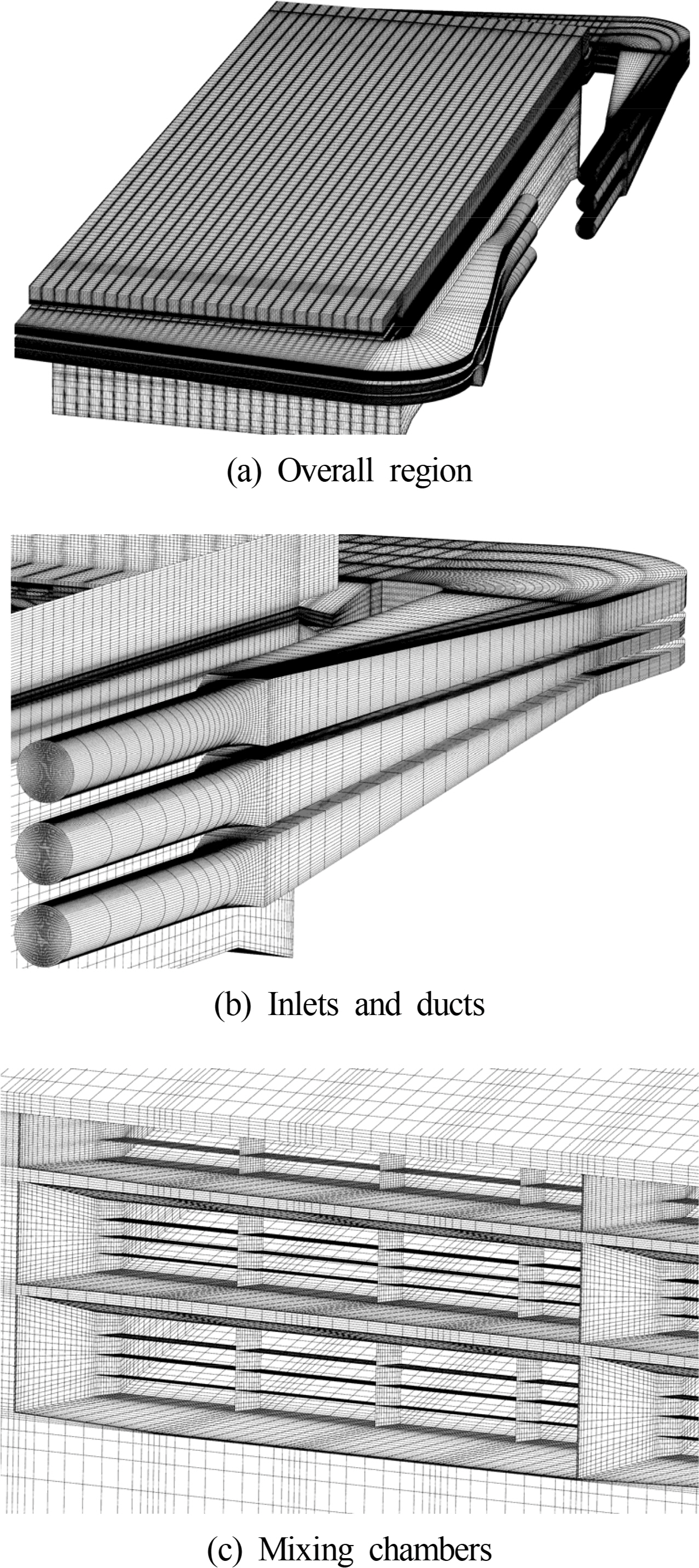
The three less important lower channel layers were not included in the grid in order to reduce the complexity of the three-dimensional simulations and to avoid a massive increase of grid points. Except for neglecting the thickness of flow-embedded control surfaces, the generated grid considers every part of the current generation system without further geometrical assumptions. As can be seen in Fig. 3, which shows the grid distribution around the main parts, the current study used a multi-block structured grid with 11.0M (million) grid points.
In this study, the flow rate of the impellers and the solidity of the screen models should be determined for the generation of uniform current. Table 1 shows the average magnitude of the axial flow velocity at each impeller face of the current channel layers. These values were determined through numerical experiments to reproduce the target current speed of 0.5 m/s on the free surface in the basin.
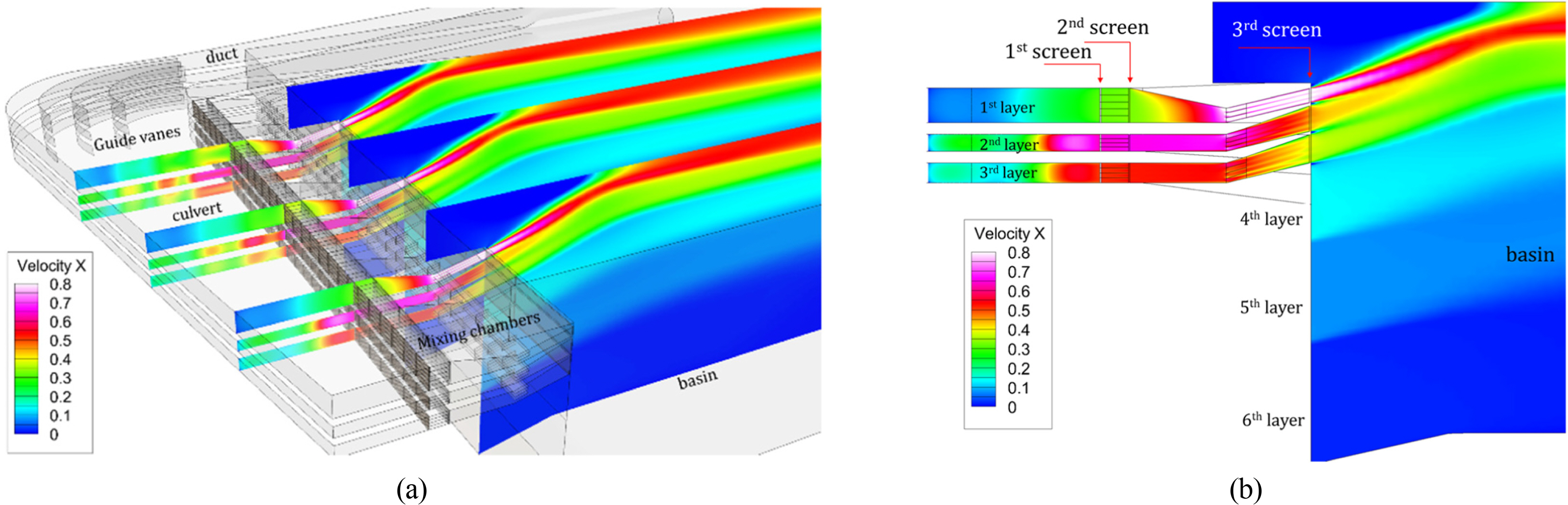
Fig. 4 shows the streamwise velocity distributions on the selected vertical planes at y=8 m, 15 m, and 27 m in the DOEB. It is seen that the flows entering the culverts after turning 90° through the ducts are significantly complicated. After the flows passed through the screens and mixing chambers, a current with stratified flow velocity distribution in the depth direction was generated in the basin. The solidity values of the three screens from a previous study (Park et al., 2014)are shown in Fig. 4(b). The values required to generate the desired uniform current in the basin were determined to be 0.5, 0.83, and 0.5. A re-circulation flow region developed near the free surface above the 1st channel layer, and its length spanned 5.9 m from the exit of the channels. However, the effects of the re-circulation flow are not expected to be significant since the location of the model test zone is 50 m from the current channel exit.
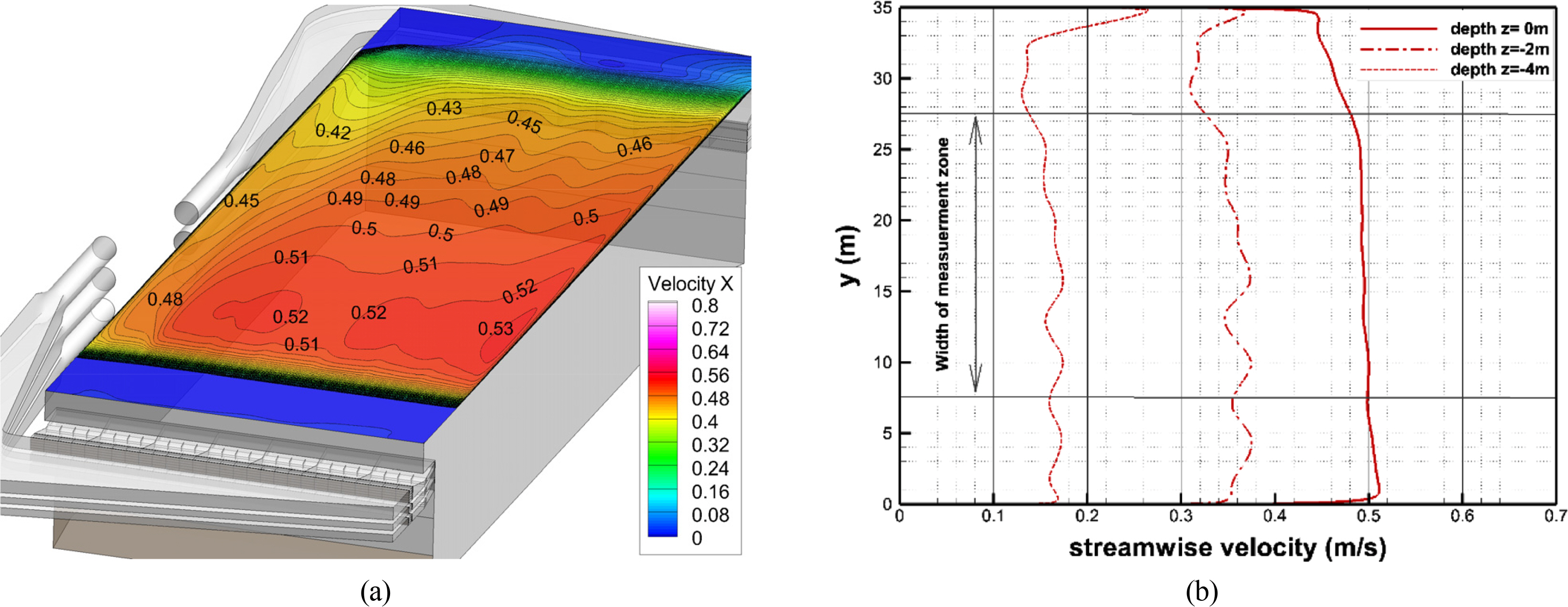
Fig. 5 shows the streamwise velocity distribution of the generated current on the free surface and its profiles extracted at x = 50 m in the y direction. As shown in Fig. 5(a), re-circulation flow regions were formed in the upstream and downstream parts of the basin. The current speed slowed as the flow went downstream of the basin, but sufficiently constant current distribution was obtained over the measurement zone.
As shown in Fig. 5(b), the predicted streamwise velocity profile on the free surface at x = 50 m satisfies the extreme current speed target of 0.5 m/s. On the other hand, the uniformities of the velocity profiles below the free surface were slightly low. This can be overcome by using higher solidity, but it causes an increase in the head loss of the current pumps. In model tests, it is necessary to investigate the effects of the non-uniformity of the current below the free surface according to the draft of offshore structure models.
Fig. 6 shows a comparison of the vertical current profile. The target current profile in the figure was designed as an extreme case by referring to field data. The predicted profile was extracted in the z direction in the middle of the model test zone at x = 50 m and y = 17.5 m. The water depth influenced by the three upper current channel layers that were directly considered in the grid was about z = −5.8 m. Below this depth, the current profile was generated by a constant velocity inlet condition with an inclined angle imposed at the inflow section of each of the three lower current channel layers. Within the design capacity of the pump, the current generation system reproduced the design extreme current profile well and showed good agreement. Table 2 shows the calculated results of the head loss of the current channel at the design flow rate. The maximum head loss value was used for the pump capacity and impeller design.
2.2 Design of Current Generation System
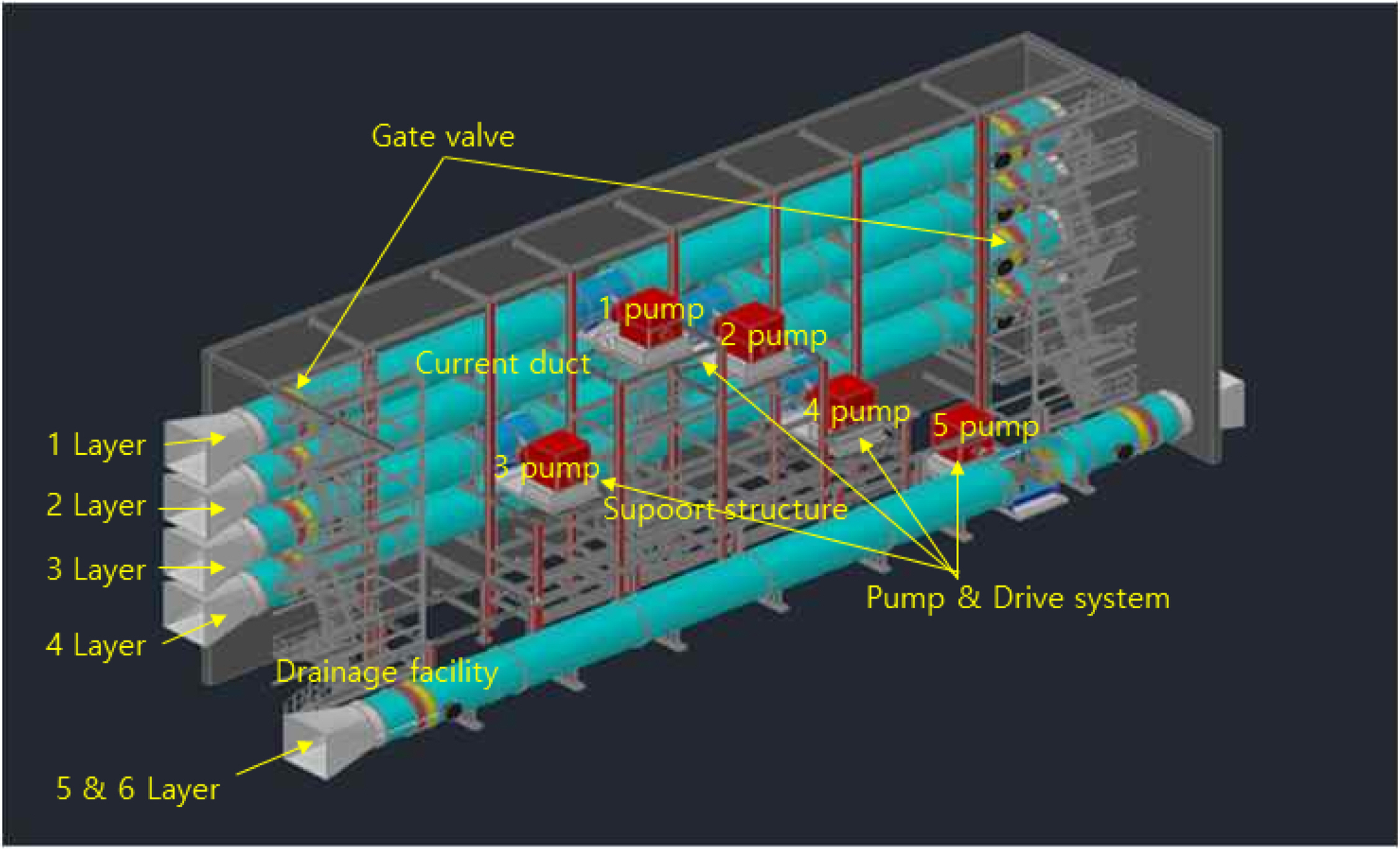
The current generator is composed of a six-layer water channel aligned vertically to realize arbitrary current spatial distribution, and five current pump facilities (combining the lower current channel). A conceptual diagram of the current pump facility is shown in Fig. 7, and it is composed of a current duct, facility support structure, pump and drive system, drainage facility, electric unit, and operation control system. The current duct is a steel structure with a circular cross-section of sufficient strength and a support structure to withstand the self-weight and pressure of the basin. It ensures uniform circulation flow transfer, and each duct is connected in the form of a bolted flange. It was placed such that the waterway could be blocked with a gate valve. The current duct arrangement was designed in series with the two rows (five and six layer) forming one layer and the four layers being without inflections to minimize possible head loss.
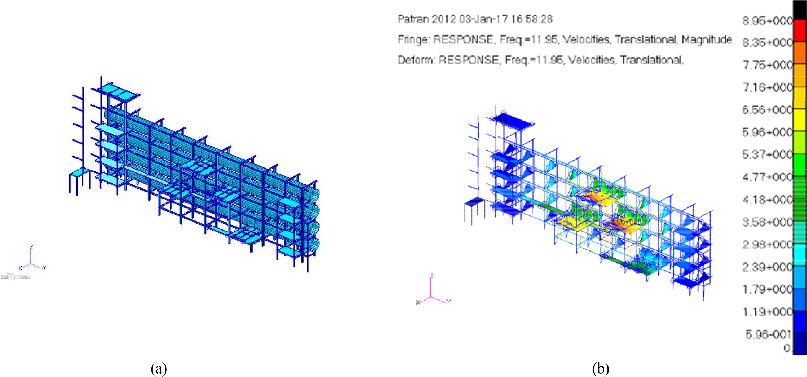
The supporting structure supports static loads generated by the self-weight of the motors, impellers, and current ducts (when the generator is switched off), dynamic loads generated by driving the motors and impellers, and the duct flow, The supporting structure prevents damage to the duct system due to thermal deformation. For analyzing the strength of the supporting structure, as shown in Fig. 8, static and dynamic strength analyses were performed. In addition, an earthquake analysis was performed on the facility’s supporting structure to verify the stability of the design values.
The figure on the left of Fig. 8 shows a model for structural stability analysis of the support structure arranged in the vertical direction from duct 1 to duct 4. Analysis was done modeled through MSC/PATRAN. In this case, 1,081 elements were used, and 70 nodes were used. The boundary condition of the vibration analysis model is the same as in the static analysis, and a constraint condition of 6-DOF motion for translational and rotational motion was applied to the part fastened to the basic anchor bolt.
The primary natural frequency obtained through natural frequency analysis of the supporting structure was 3.7332 Hz, and the main natural frequencies were 8.6308 Hz, 9.1378 Hz, 10.183 Hz, 10.454 Hz, 11.055 Hz, 11.544 Hz. 11.704 Hz, 11.89 Hz, 14.027 Hz, and 14.302 Hz. Among them, the result for 11.95 Hz is shown in Fig. 8 (right). Through vibration response analysis, the maximum displacement in the 1–5 Hz section were 0.053 mm, which was less than 1.0mm, which is the standard for DNV steel structures and satisfies the stability standard. In the case of the 5–15 Hz section, the maximum speed is 8.95 mm/s, which is lower than the 30 mm/s standard for DNV steel structures, which satisfies stability.
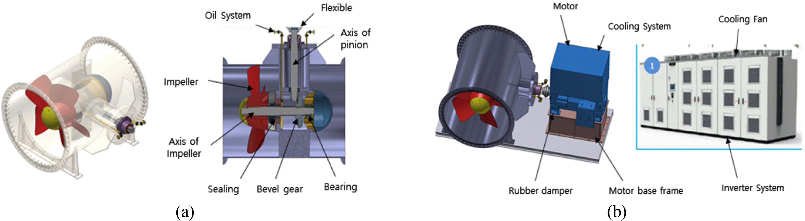
The current pump used are an axial pump that accelerates the circulating fluid. As shown in Fig. 9, it comprises an impeller, gear housing, bevel gear, impeller shaft, pinion shaft, flexible coupling, bearing, sealing, and lubricant system, and has a structure that can be completely sealed.
An axial-type impeller was selected based on the particular speed. The impeller was designed to have the best efficiency, good cavitation, and low vibration performance, and an azimuth thruster was selected because it has efficient maintenance. The number of blades was selected as five to absorb the high power density and avoid a resonance with a “+”-type stator system. Design conditions were selected according to the target profile (waterway capacity of 14.9 m3/s and required head loss of 1.33 m) and to absorb the motor power. Two types of impellers were designed to ensure suitability for different loads due to the head loss across the flow layer. The first impeller type was designed for the second and third layers, and the second impeller type was designed for the first, fourth, and fifth layers.
The performance of the pump was predicted using a lifting-surface theoretical analysis, and the pitch and camber distribution were determined. The performance of the impeller in the channel was calculated based on the lift surface theory and CFD. The CFD turbulence model and discrete scheme were the same as those used for the aforementioned current channel analysis.
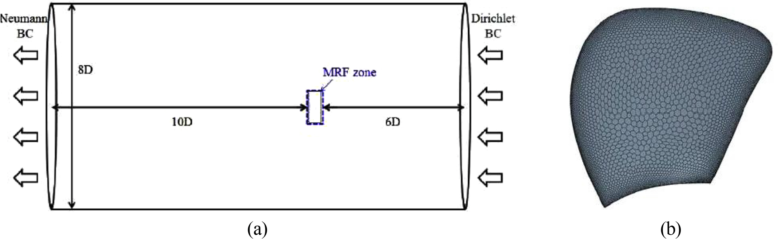
Fig. 10 shows the computational domain and grid distribution on the impeller surface for the single-impeller performance analysis. A hybrid mesh technique with polyhedral and trimmed meshes was employed due to the complex shape of the impeller. The polyhedral mesh was applied to the MRF rotating region, including the blade, while the trimmed mesh was used for the remaining region. To simulate the turbulent boundary layer, five prism layers were generated on the blade surface, and
y P + ≈ 30
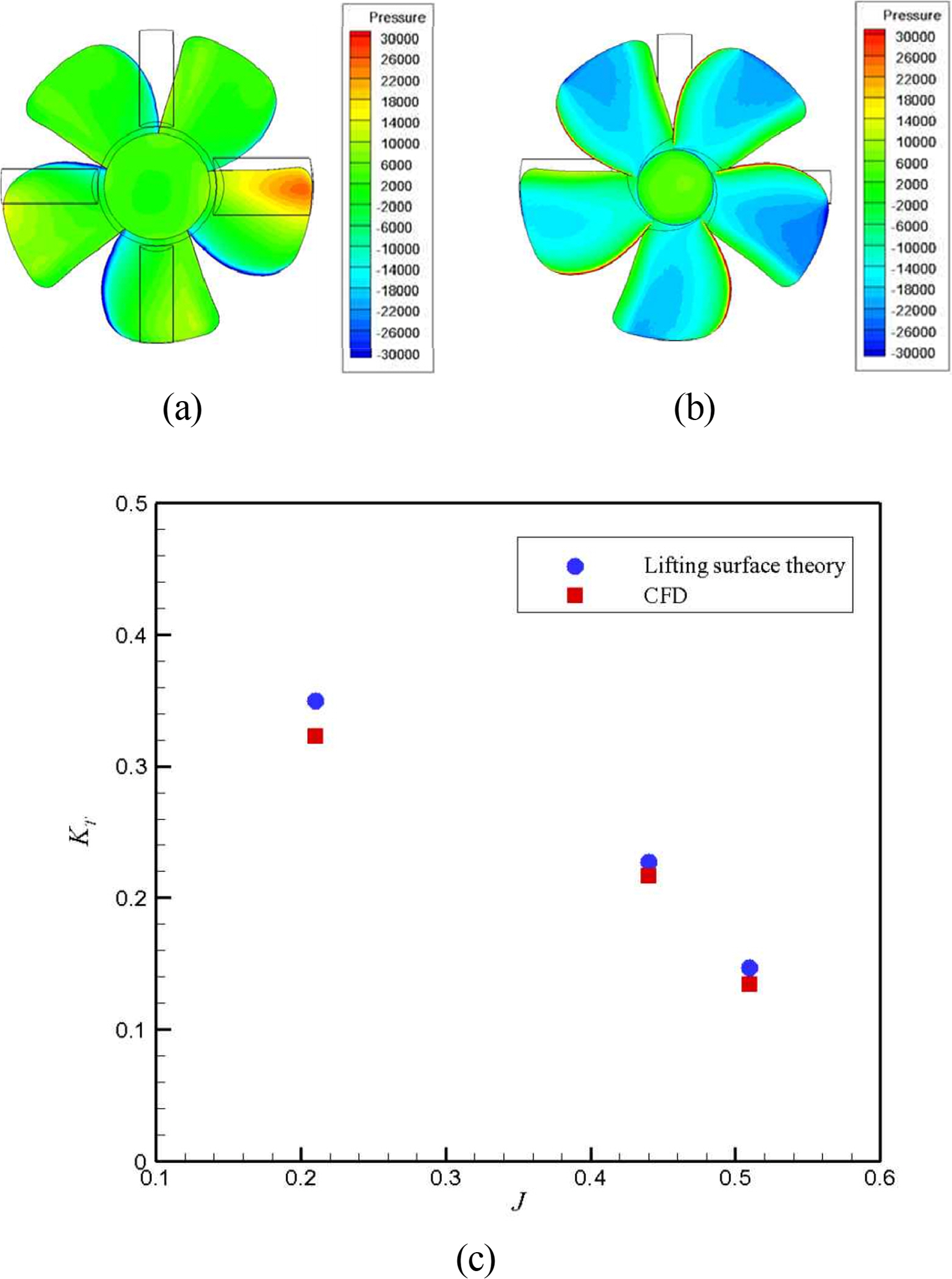
Fig. 11(a) and Fig. 11(b) show the pressure distributions on the pressure and suction sides of the blade, which were obtained after the impeller thrust and torque converged. Similar to the pressure distributions of a general thruster, the pressure increases at the leading edge of the blade while gradually decreasing toward the trailing edge. Fig. 11(c) presents the result of the single-impeller performance in terms of the thrust coefficient and advance ratio. The results of the non-viscous-based lift surface theory and the CFD analysis show the same physical trend. Based on this result, it can be confirmed that the CFD analysis results show similar accuracy to the lift plane theory. Table 3 shows the flow rates and the delivered horsepower (DHP) at various impeller revolutions per minute (RPM) for channel 1 with impeller 2 and for channel 2 with impeller 1.
2.3 FAT (Factory Test) of Current Generation System
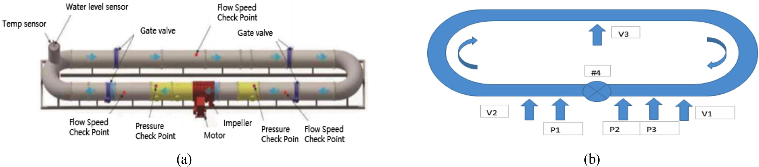
Before installing the current pump, an FAT of the current pump was performed as shown in Fig. 12, to verify the performance and durability of the current pump. The FAT consisted of a leak test for the major parts, a pressure test for each section, and a performance test for the pump. The pump performance test was divided into 5 stages based on the different motor load values: 1/4, 2/4, 3/4, 4/4, and 11/10 times the initial motor load. The number of rotations for each load and, required shaft horsepower current, voltage, coolant temperature, and performance were analyzed by measuring the temperature and lubricant temperature.
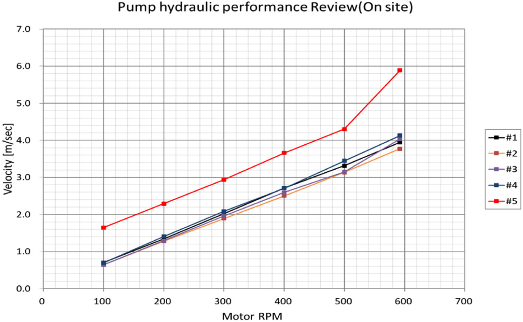
As shown in Fig. 12 (b), the flow rate was measured by an ultrasonic system at three positions, V1 was at the inlet side, V2 was at the outlet side, and V3 was diametrically opposite the impeller. The measured flow rates at V1 are relatively low because V1 is far downstream from the impeller. The flow rate according to the RPM change was analyzed with respect to the FAT result of the pump performance, as shown in Fig. 13. The measured flow rates, except for pump #4 were stable for the various RPMs and are similar to the predicted flow rates.
The delivered horsepower (DHP) was obtained based on the motor output voltage and current obtained during the pump performance FAT. The DHP curves of impellers are shown in Fig. 14. These curves are in good agreement with the predicted value, which is at table 3 (impeller 2), dependent on the accuracy of the flow rates in FAT and impeller efficiency.
2.4 Installation and Testing of Current Generation System
The current generation system was installed in the current pump room of the DOEB, and all the inspections and durability tests were performed on the major components. Safety checks were conducted on the shafting alignment, electrical parts, and installation structures, which are the main components of the on-site installation of the current generation system. The shafting alignment is very important for stably driving the current generation system for a long duration. For this purpose, the single and interlock drives (with 5 pumps simultaneously) drives were performed for more than 8 h per day for 2 weeks, and the alignment status was checked by separating the shafting system.
After the completion of the stability check of the current generation system, a single pump performance test of pumps 1–5 was conducted, and the pump performance was reviewed by interlocking five pumps, as shown in Fig. 15, By interlocking five pumps. The performance of the pump was maintained at a maximum flow rate of 4 m/s. This result exceeds the CFD prediction result for the pump output flow rate for forming the target vertical profile as shown in Table 1. And there was no significant difference in the flow rate performance of the pump in the single and interlocking drives. However, an increase in the flow rate of pump #5 was observed during the FAT. This is because pump #5 is responsible for current channels 5 and 6 of the DOEB.
3. Analysis of the Current Characteristics in DOEB
3.1 Characteristics of Flow Rate of the RPM Current in the Current Generation System
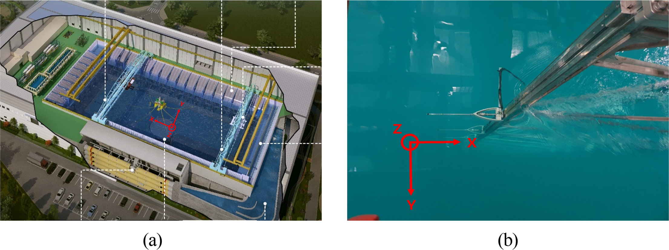
According to the impeller drive of the DOEB current generation system, current is generated in the DOEB test area through the waterway. The experimental area of the DOEB is near the middle area of the DOEB, and the test area is set as shown in Fig. 16 to analyze the current velocity from the water depth.
The result of measuring the flow rate in the DOEB by increasing the RPM of the current pump facility is shown in Fig. 17. It can be seen that the flow rate is 0.56 m/s at the maximum RPM of the current pump facility, which exceeds the design target flow speed of 0.5 m/s. Based on these flow velocity results, the initial driving RPM can be estimated when the current velocity is reproduced for the following model test.
3.2 Spatial Area Characteristics of Current in DOEB
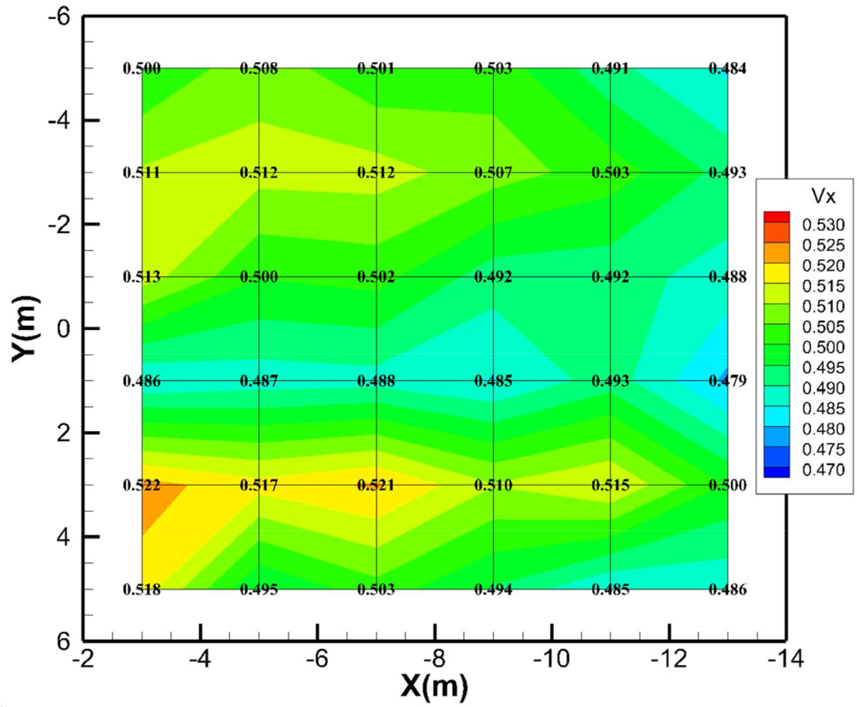
To investigate the distribution of the current velocity in the DOEB, the towing carriage was used, and the current velocity was measured as shown in Fig. 18. The error range of the average flow velocity distribution in the test area of the model test (10 m (width) × 10 m (length)) was within 5%. This confirms that the DOEB current channel waterway and the several turbulence control devices are working effectively.
As shown in Fig. 19, the turbulence intensity (T) was examined based on the equation obtained by Bas Buchner (Buchner and Wilde, 2008).
where σ is the standard deviation of the velocity fluctuations, and V is the mean velocity.
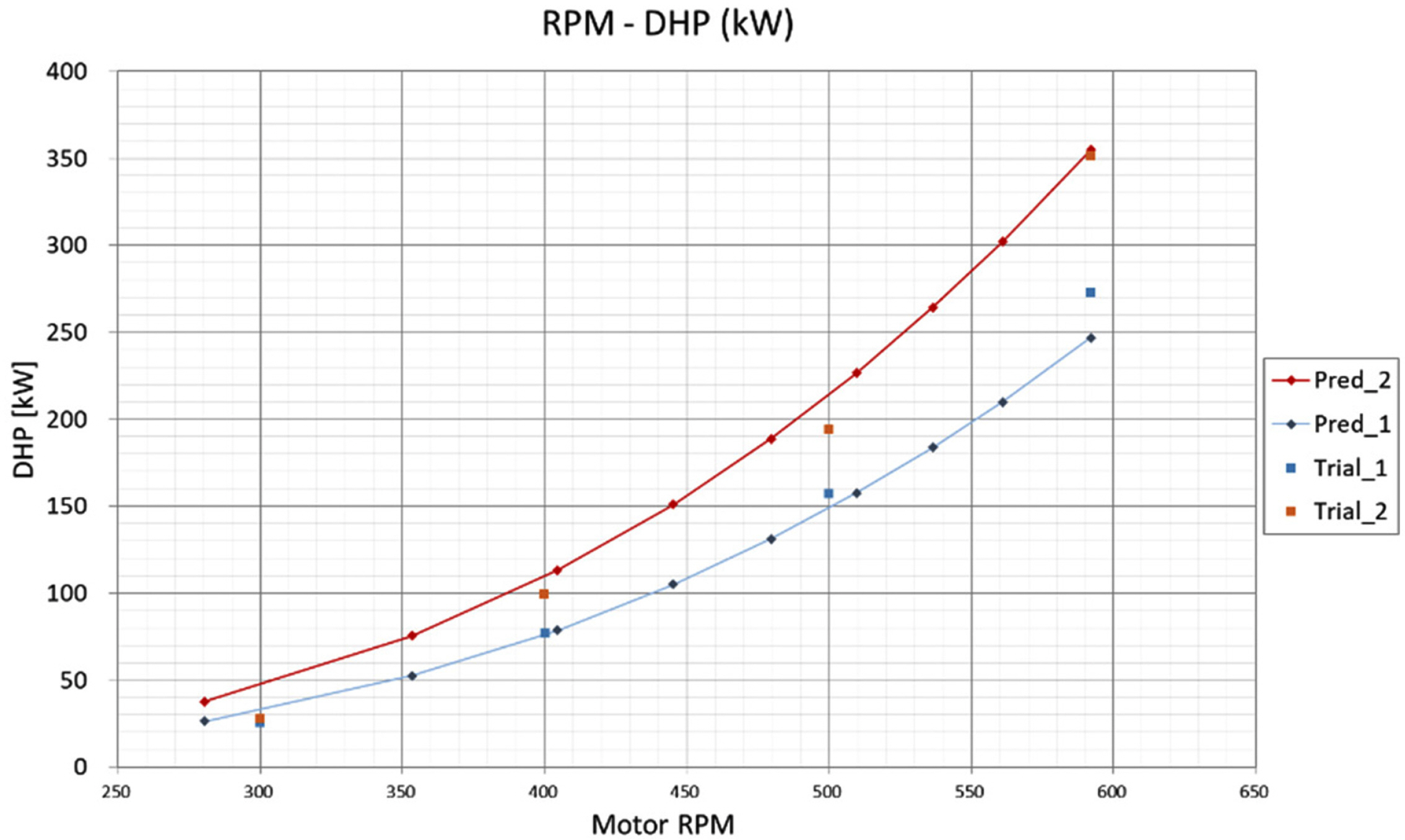
It can be seen that the turbulence intensity of the current near the test area of the DOEB is 7–8%. A turbulence intensity improvement test was planned through a solidity change test of the turbulence grid (SUS screen) at the outlet. The performances of pump #1 and pump #2 plays a significant role in obtaining the target current velocity in the test section. Fig. 20 shows the DHP curves for pumps #1 and #2 during the performance test, and they are in good agreement with the predicted value.
4. Conclusions
In order to design the current generator in the DOEB of KRISO, a 3D numerical analysis was performed to evaluate the hydrodynamic performance of the current channel of the current generator. Based on the analysis results, the number of screen devices installed in the current channel, location of the installation, and distribution of current according to the solidity were reviewed, and the maximum flow velocity of current in the surface layer was obtained. The head loss of the current channel was also obtained.
The main components of impellers were designed based on the hydrodynamic performance of the current channel and verified through an FAT and pump hydraulic performance test in the DOEB. Finally, by measuring the characteristics of current generation in the DOEB test area, it was confirmed that the design performance target was satisfied. Further research will be conducted on the development of a turbulence control device for improving the current turbulence intensity and the current distribution characteristics in the DOEB data based on the depth.