


1. Introduction
Offshore drilling refers to a mechanical process of drilling mud to extract petroleum or natural gas through a wellbore in the seabed. The mud is a mixture of oil (or water) and bulk materials (barite, bentonite, polymer, etc.) and it has high viscosity. It can be used to remove cuttings, provide hydrostatic pressure, and cool down or lubricate the drill bit. There are many different types of facilities where offshore drilling operations take place, and the core system is a drilling system that is mainly maintained by mud-handling and bulk-handling systems.
When a drilling operation is being performed, many physical and chemical changes occur in the wellbore. In order to handle many changes in the well conditions and maintain the drilling process, bulk additives are added to drilling mud through a mixing system. Examples of additives include bentonite for increasing the density of the drilling mud, barite for increasing the viscosity, polymer for chemical control, surfactants, etc. In this process, a mud agitator performs the function of mixing both the mud and bulk, which are pre-mixed in a mud tank, and the homogeneous material properties are maintained using the swirling motion of a mechanical impeller. The achievement of required material properties through the mud agitator is essential to stabilize a drilling system. Thus, it is important to analyze the multi-phase flow and system and guaranteeing safety.
There have been some experimental and numerical investigations for the design of agitators, including fundamental experiments regarding the change geometric shape of the impeller (Nagata et al., 1959), performance of agitation with various sizes of the impeller (Nienow, 1997), and experiments in regard to change torque and position of impellor with 45° pitched blades (Chang and Hur, 2000; Choi et al., 2013). Experimental measurement was done using a laser Doppler velocimeter (LDV), and numerical simulation was done for the flow patterns in an agitator relating to its geometric shape and power of agitation (Kumaresan and Joshi, 2006). Unsteady numerical simulation was done with a free surface in an agitator (Ahn et al., 2006), and a solid-liquid multiphase simulation was done using a granular flow model in the commercial software ANSYS-Fluent for multiphase interaction (Darelius et al., 2008). Numerical simulations were done to predict the solid particle distribution in an agitator using various baffle types (Kim et al., 2009) and various impeller speeds (Wadnerkar et al., 2012), and a numerical simulation was done for particle distribution in an agitator using the commercial software STAR-CCM+ (Lo, 2012; Kubicki and Lo, 2012), etc..
In summary, many experimental investigations have been performed to design an agitator and predict the solid particle distribution in a stirred tank using an experiment, and it seems to be difficult to predict the mixing performance and to conduct an experiment directly for high-viscosity fluids. As an alternative way, computational fluid dynamics (CFD) simulations have also been carried out for predicting the performance of an impeller and the distribution of solid particles inside a mixing tank. However, for more practical application of a mud agitator to some equipment in an offshore plant, a multiphase simulation of solid-liquid flow should be performed with high-viscosity mud inside the tank.
In the present study, the numerical simulation of swirling and liquid-solid multiphase flow around a mechanical agitator system was carried out to investigate the distribution of bulk particles in a system using commercial CFD software, STAR CCM+ ver.8.04, based on an Eulerian-Eulerian approach. First, for verifying the CFD tool, water mixing problems for a model-scale agitator were simulated with various turbulence models, and the results of the simulation for the velocity components around the impeller were compared to those of experiments performed by Guida et al. (2009) and Guida (2010). Next, the liquid-solid multiphase flow in a mud agitator was simulated with different multi-phase interaction models, and both the velocity profile and solid concentration were compared with the experiments (Guida et al., 2009) and another numerical simulation (Kubicki and Lo, 2012). Finally, the liquid-solid multiphase flow in a mud agitator was simulated under properly adopted simulation conditions. The prediction of the mixing time and distribution of bulk particles in the mud agitator are discussed.
2. Numerical Formulation and Conditions
2.1 Governing Equations and Numerical Modeling
The governing equations for an incompressible and viscous flow involving multiple phases are the continuity and Reynolds-averaged Navier-Stokes (RaNS) equations. To solve the liquid-solid multiphase flow, governing equations were modified with the volume fraction of each phase, and momentum transfer and internal force terms were added to the right hand side (RHS) of the RaNS Eq. (2) as follows:
where α is the volume fraction, ρ is the density, t is time, u is the velocity vector, p is the pressure, τ is the stress, τt is the turbulent stress, g is the gravity acceleration, M is the momentum transfer term between the different phases, Fint is the internal forces, and the subscript i indicates the type of fluid.
Components of multiphase interaction models composed of momentum transfer and internal force terms on the RHS of Eq. (2) were modeled in the same manner as Kim et al. (2017) and CD-Adapco (2014). In order to consider the momentum exchange at the interface, the drag, lift, and turbulent diffusion forces for multiphase flow are introduced in the present study. For the drag force, we used Gisdaspow’s model (Gidaspow, 1994) and Syamlal and O’Brien’s model (Syamlal and O’Brien, 1989), which consider the behavior of solid particles. In the case of Gisdaspow’s model, the linearized drag coefficient can be obtained by the following equation (3):
Here, αp is the volume fraction for solid phase, which was obtained as 0.2 through an experiment. μc is the viscosity of the liquid phase, ρc is the density of liquid, l is the average diameter of particles, αc is the volume fraction for liquid, and ur is the relative velocity between adjacent phases. The drag coefficient CD is corrected by a correlation equation from Schiller and Naumann and is written as Eq. (4):
where the Reynolds number for the dispersed phase can be expressed in Eq. (5):
Similarly, Syamlal and O’Brien’s drag model is obtained from the measured value of the terminal velocity in the bed where solid particles are deposited and is calculated as Eq. (6):
where umf is the minimum fluidization velocity, and CD is the drag coefficient of the solid particle group, which is presented as Eq. (7):
Here, CDs is the drag coefficient of a single solid particle and is given in Eq. (8):
where Res is the Reynolds number of a single solid particle in Eq. (9), and Vr is the ratio of the terminal velocity of the single particle in Eq. (10) and the total particles:
where μp is the viscosity coefficient of the solid phase, and ρp is the density of the solid phase.
The lift acts in the direction perpendicular to the relative velocity between solid and fluid particles and can be calculated as Eq. (13) by Auton’s formula (Auton, 1987):
where u is the velocity of fluid, and CL is the lift coefficient. In the case of the lift coefficient, the default value is set to 0.25, but in this study, a value of 0.1 was used because it is suitable for small-sized particles according to Ekambara et al. (2009).
Next, the turbulent diffusion force due to the interaction between solid particles and fluid eddy is considered as shown in Eq. (14):
where σp and σs are the turbulent Prandtl numbers of the solid and fluid, respectively, and both are set to a value of 1. Additionally, νpt and νst represent the kinematic viscosity of the solid and fluid due to turbulence, respectively. Inside the solid phase, a pressure force between the solid phases acts when the distribution of the solid reaches the maximum distribution. In order to consider the pressure of the solid, in this study, the granular pressure model was used, as represented by Eq. (15):
where Pp is the solid pressure, μp is the effective granular viscosity, I is the isotropic tensor, and ξp is the bulk viscosity.
In the granular pressure model, the interactions between particles are considered by dividing them into several cases. First, in the case of the kinetic regime, the collision between particles is defined by the distribution function g0 of Ding and Gidaspow (1990) if the particle distribution is lower than the maximum distribution criterion as Eq. (16):
where αp is the particle volume fraction, and αp, max is the maximum particle volume fraction.
The distribution function go is used to calculate the granular temperature θp, which determines the effective granular viscosity. The effective granular viscosity is composed of the collisional (C) and kinetic (K) contributions (Gidaspow, 1994) as given in Eqs. (17)∼(19):
The formula of Schaeffer (1987) was used for the frictional regime, in which the distribution of solid particles is close to the maximum distribution criterion. In this case, the solid pressure and effective granular viscosity can be written as Eqs. (20)–(21). In this case, ϕ is given as 25° from Schaeffer (1987). In addition, the maximum distribution criterion for rigid spherical solid particles is applied based on the representative value of 0.624 obtained from an experiment.
2.2 Geometric Shape and Ggrid System
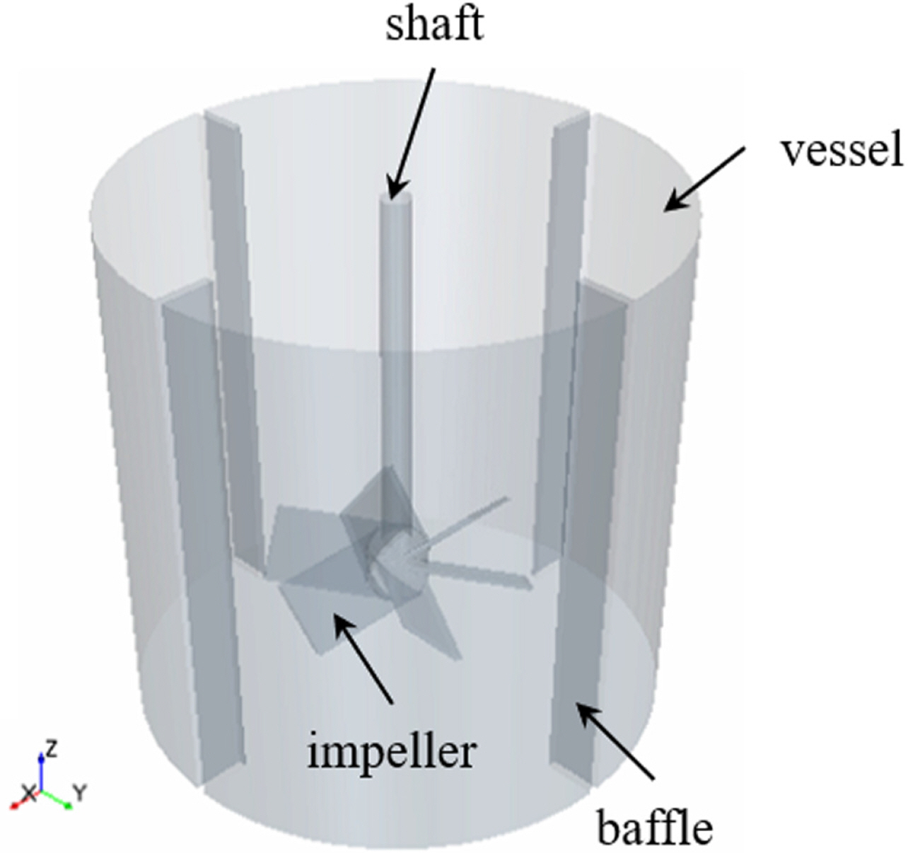
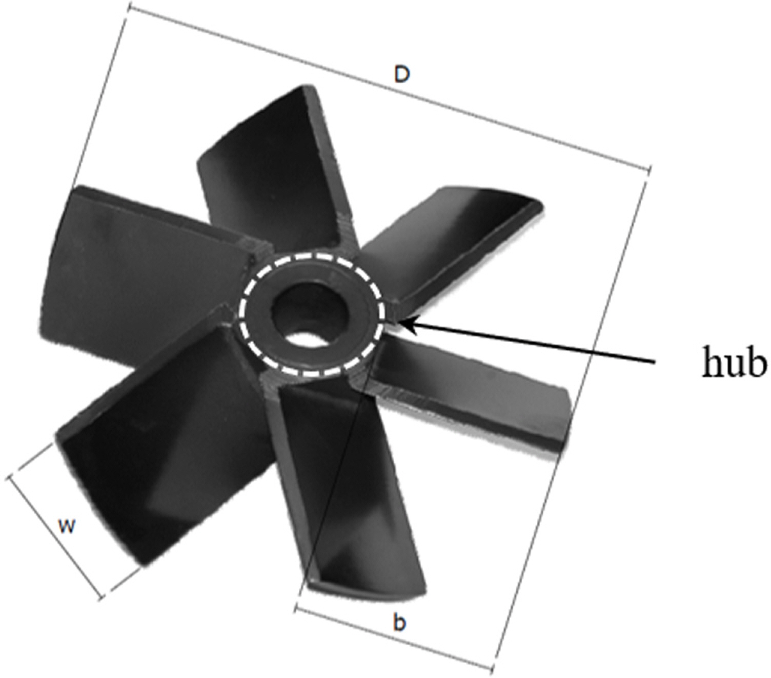
For the verification of the CFD tool, STAR-CCM+, firstly, the single-phase swirling flow in an agitator was simulated and compared with an experiment (Guida et al., 2009). The experiment was conducted in a model-sized cylindrical tank with 4-plate baffles and a 45°-pitch 6-blade impeller, as illustrated in Fig. 1. The connection between the hub and blades of the impeller was referenced from Guida et al. (2009), as shown in Fig. 2. The detailed dimensions of geometric shapes are summarized in Table 1. In the experiments, the rotation of the impeller was set to 360 rpm. Salt water with a density of 1,150 kg/m3 and viscosity of 0.0045 Pa·s was used as the working fluid. The Reynolds number was calculated based on the maximum diameter of the impeller as about 106.
The grid system shown in Fig. 3 was generated almost automatically by an algorithm in STAR-CCM+. For solving the rotary motion of the impeller, a cylinder-like rotational region including both the impeller and its shaft was designated using polyhedral meshes with a prism layer that has a minimum size of y+≈30. The total number of grid elements used was about 1.8 million for the turbulence model test, and 5 grid systems in the range of about 800,000–4,800,000 elements were used for the grid convergence test.
2.3 Boundary Conditions
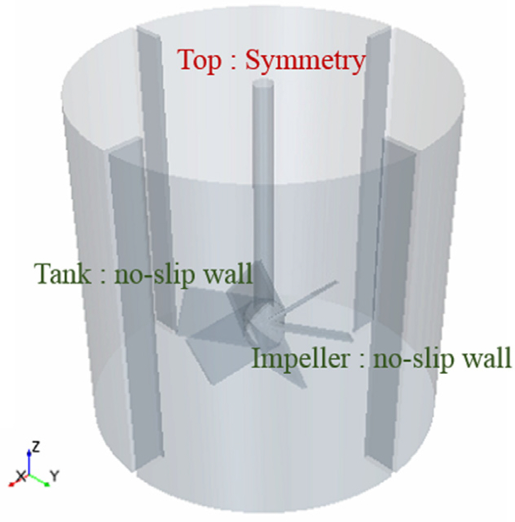
The boundary conditions for the simulation are defined in Fig. 4. A symmetry boundary condition was adopted at the top of the tank, assuming that the free-surface motion does not significantly affect the entire flow field. Other wall boundaries including the impeller were given no-slip wall conditions. The rotary motion of the impeller was applied by introducing a rigid body motion (RBM) model that directly rotates the rotational region inside the grid system. The time step in the simulation was set to 0.001 s in consideration of the rpm of the impeller.
3. Simulation Results
3.1 Verification of Single-phase Swirling Flow Around Agitator
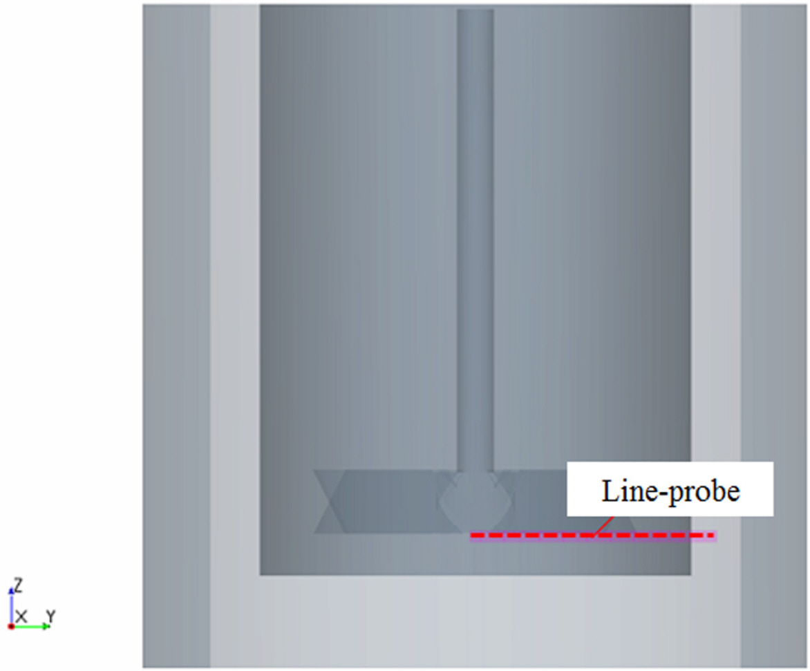
Numerical simulations for single-phase water mixing in an agitator were performed with various turbulence models to verify the applicability of the commercial software STAR-CCM+. The software can cope with the turbulent swirling flow generated by the agitator inside a cylindrical tank. The simulation results regarding the velocity components around the impeller were compared to experiments (Guida et al., 2009; Guida, 2010). In the present simulation, as shown in Fig. 5, the time-averaged velocity components were measured along the probe line just below the impeller after the flow field reached quasi-steady state.
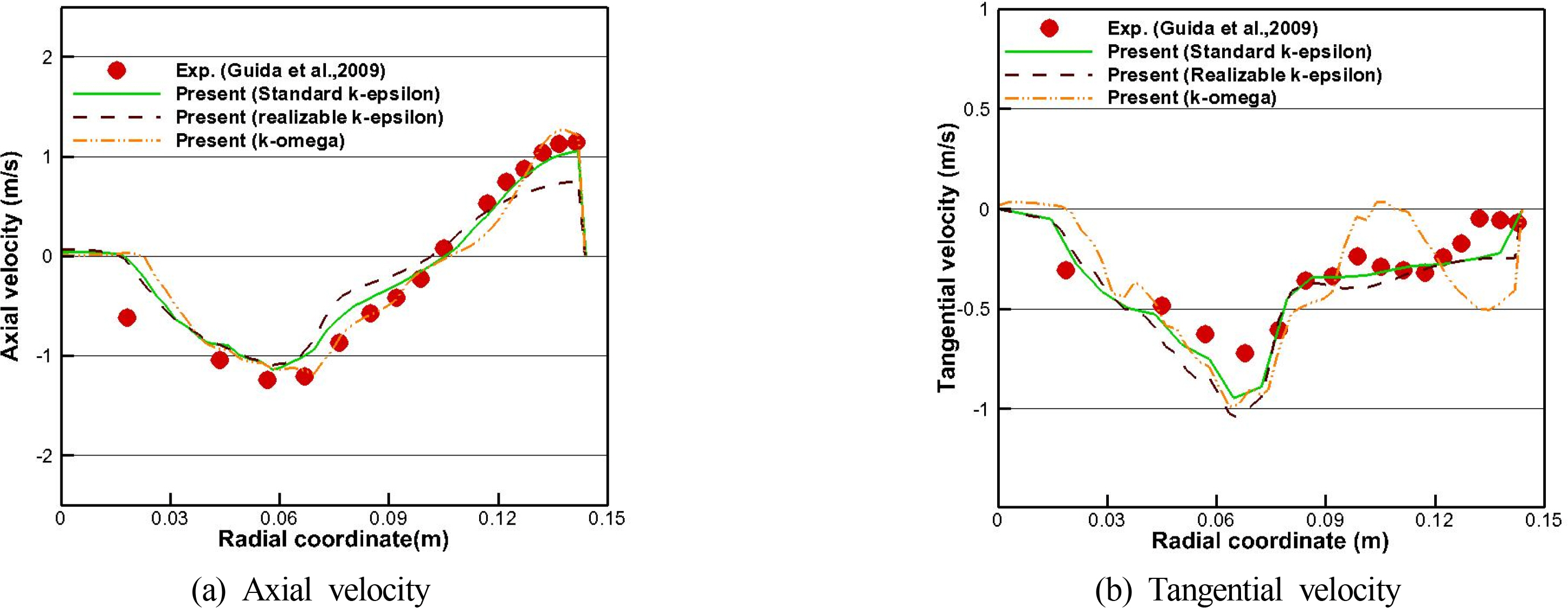
First, turbulence models based on 2-equation models were tested: the standard k − ∊ (SKE), realizable k − ∊ (RKE), and k − ω models (KW) models. The initial conditions for turbulence in the flow field for all subsequent cases were turbulence intensity (TI) = 0.01 and turbulent viscosity ratio (TVR) = 10. Fig. 6 shows the time-averaged profiles of the simulated axial and tangential velocities compared to the experiments. Similarly, in both the simulation and experiment, the magnitude of the velocity tends to increase toward the end of the blade with a radius of 0.072 m and then gradually decreases. However, it was found that the tendency of the velocity profile is slightly different between the simulation results depending on turbulence models employed in the simulation. It seems that all of the turbulence models cannot predict accurately the peak value of a tangential velocity.
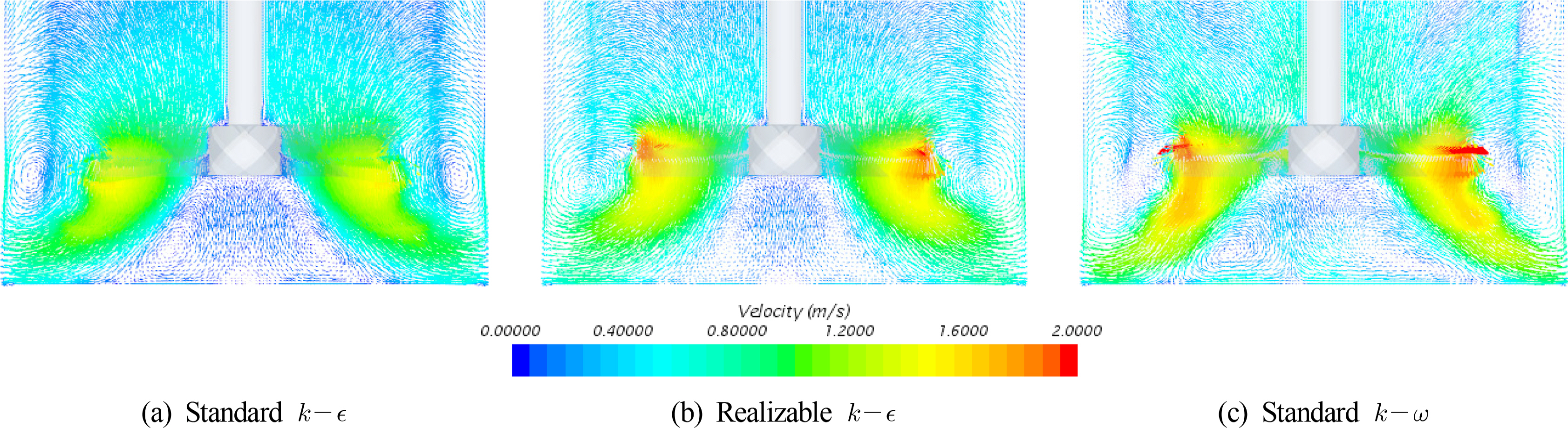
In the vector field shown in Fig. 7, it can be seen that the SKE model forms stronger vortices around the wall where the vertical baffles are attached. However, the KW model represents the small and large-scale of eddies in complicated manner in the lower part around the impeller. In the case of the real RKE model, the influence of vortices is somewhat scattered and weakened near the wall, which seems to lead to a decrease in axial velocity, as shown in Fig. 6. In the case of the KW model, small vortices around blades make different patterns of the tangential velocity compared with the experiment.
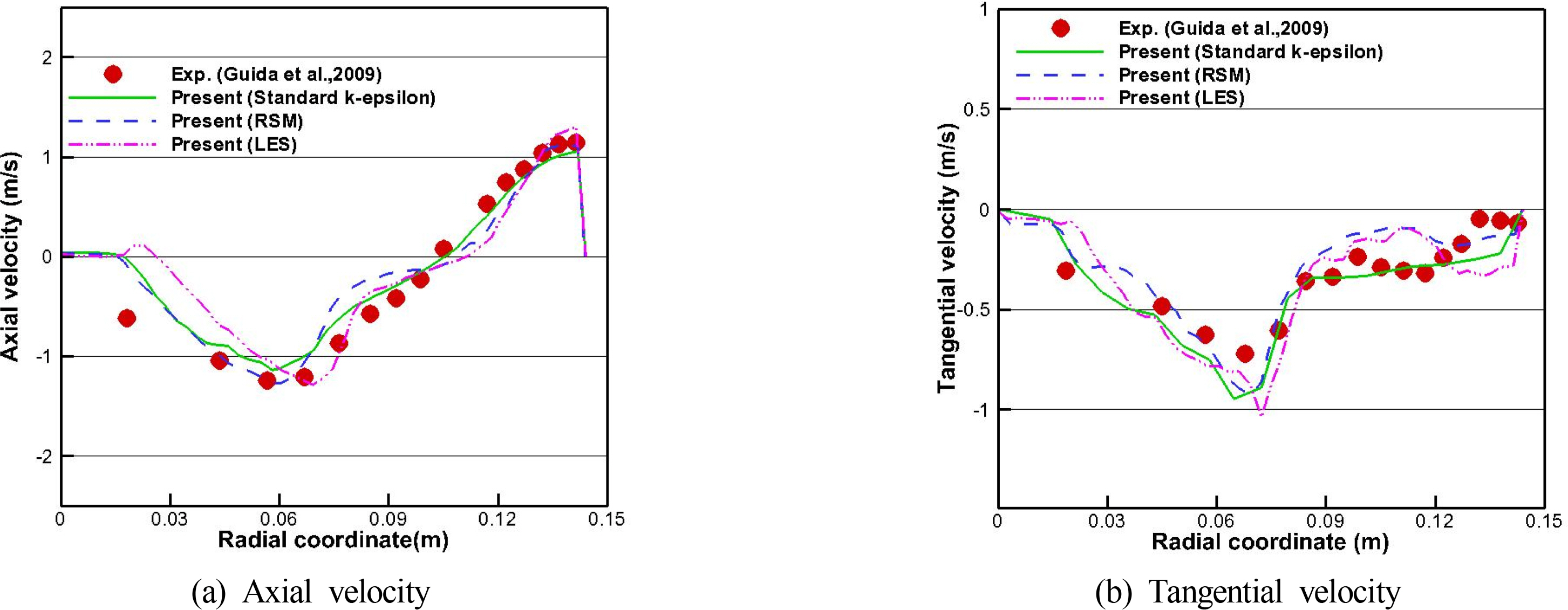
Next, numerical tests for the Reynolds stress model (RSM) and large eddy simulation (LES) were performed. In this study, the linear pressure strain and Smatorinsky models were used as sub-models of RSM and LES, respectively. The RSM is a higher-level turbulence model, and LES can resolve an ample range of both time- and length-scale eddies. In the LES, about 4.8 million grid elements were used. In Fig. 8, it seems that the results of the axial component from the RSM and LES models look more similar to the experiment at the peak value than the SKE, but the trend of the distribution after the blade ends shows a difference from the experiment.
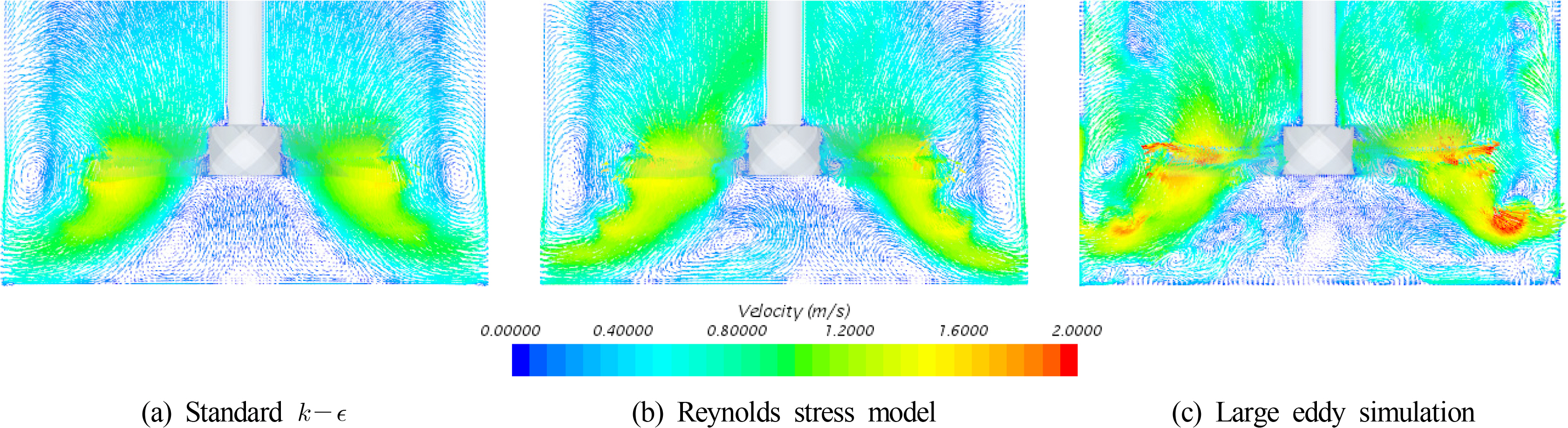
On the other hand, in the tangential component, especially in the case of the RSM and LES, there are more severe fluctuations toward the wall after the blade end. As shown in the velocity vector field in Fig. 9, it can be considered that the generation and development of more vigorous vortices in the case of RSM and LES are due to the fluctuations in the velocity distribution. As a result, both the RSM and LES models will likely require more test cases for the complemented grid system and solution setup to determine the suitability for agitation simulation. Therefore, we used the SKE, which can capture the overall average behavior of the flow field and has a relatively fast computation time.
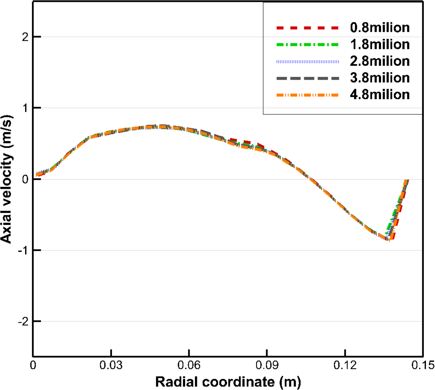
Finally, a grid convergence test was performed using SKE and five grid sizes of 0.8–4.8 million. The results of the axial velocity profile from a center position between the hub and tank bottom are shown in Fig. 10. Except for slight differences in the vicinity of the wall baffles, it seems to show a tendency to converge overall.
3.2 Verification of Liquid-solid Multi-phase Flow Around Agitator
The mixing problem of liquid-solid multi-phase flow was set in the same manner as the experimental conditions of Guida et al (2009). The flat-base cylindrical vessel has a diameter of T = 288 mm and 4 wall baffles. The inner 6-blade 45°-pitch impeller has a diameter of 0.5T and rotates at 360 rpm. The liquid was a suspension of water adjusted to a density of 1,150 kg/m3 by adding NaCl. Spherical glass beads (d = 2.85–3.30 mm) with a density of 2,485 kg/m3 were used as the solid. Initially, solid particles are evenly distributed in the space and mostly settle down from their own weight for 3 seconds. After 3 seconds, a swirling flow is generated by the rotational motion of the impeller in the agitator, and then the particles slowly start to suspend.
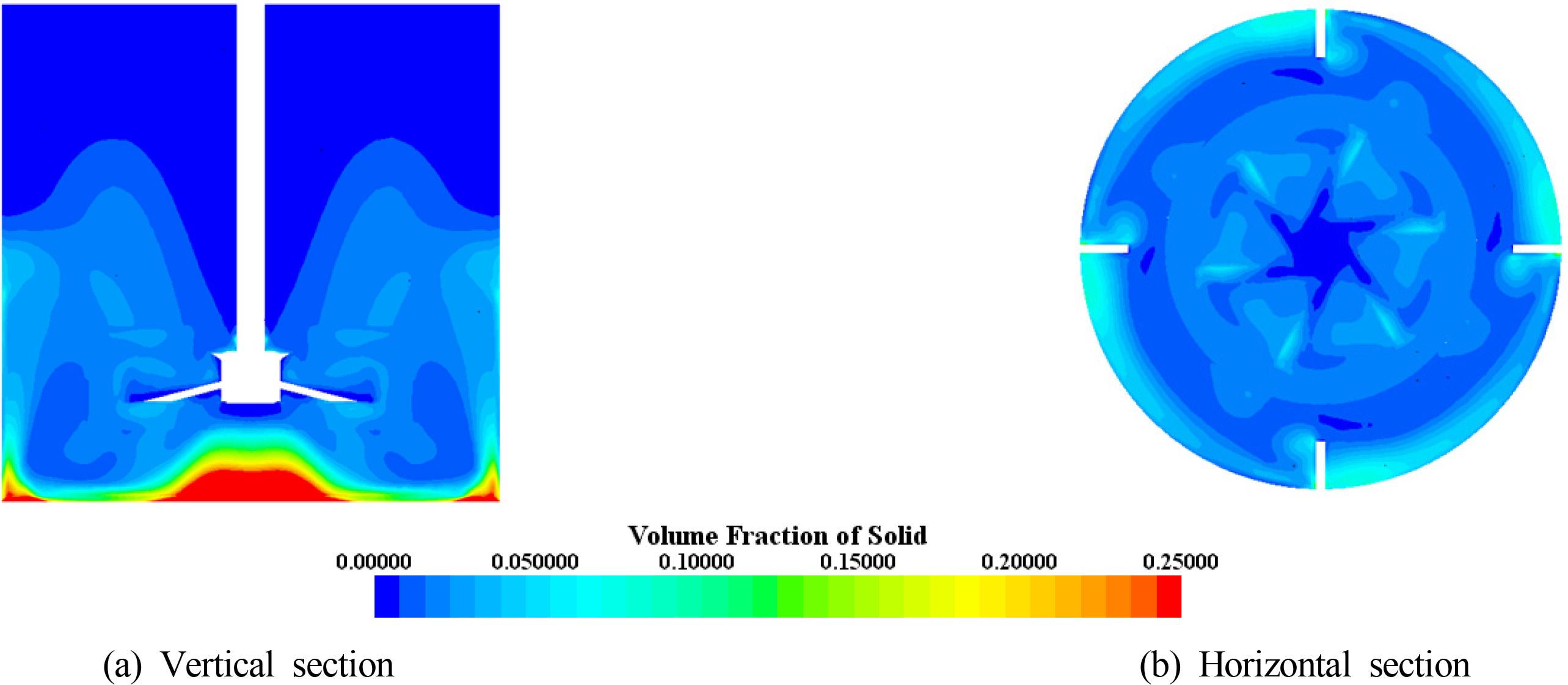
Fig. 11 shows the concentration distribution of the particles at the time when the mixed flow reaches steady state. Here, the concentration of particles refers to the volume fraction of the solid phase in a cell. A stagnation zone with a concentration higher than the average is observed below the hub and bottom corner of the wall baffles, where the flow rate is relatively low.
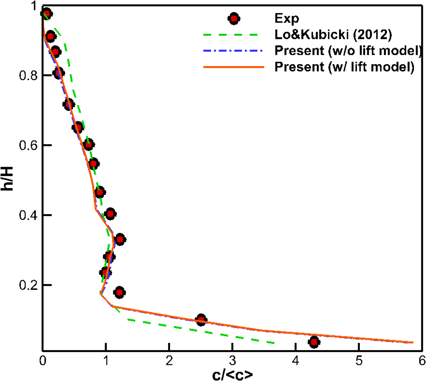
In order to find the optimal combination of liquid-solid interaction model, a multi-phase flow simulation was performed to decide whether or not to use a lift model and two different drag models (Eqs. (3) and (6)). The plane-averaged concentration according to the height was compared with the experiment by Guida et al. (2009) and the CFD simulation by Kubicki and Lo (2012). The numerical simulation by Kubicki and Lo (2012) was performed in steady state using the same CFD software (STAR-CCM+) as in this study, and the SKE turbulence model was applied. The modeling of the drag force and turbulent dispersion force for interfacial forces is the same as in this study, but for the solid pressure force, an exponential function was used instead of the granular pressure model used in this study.
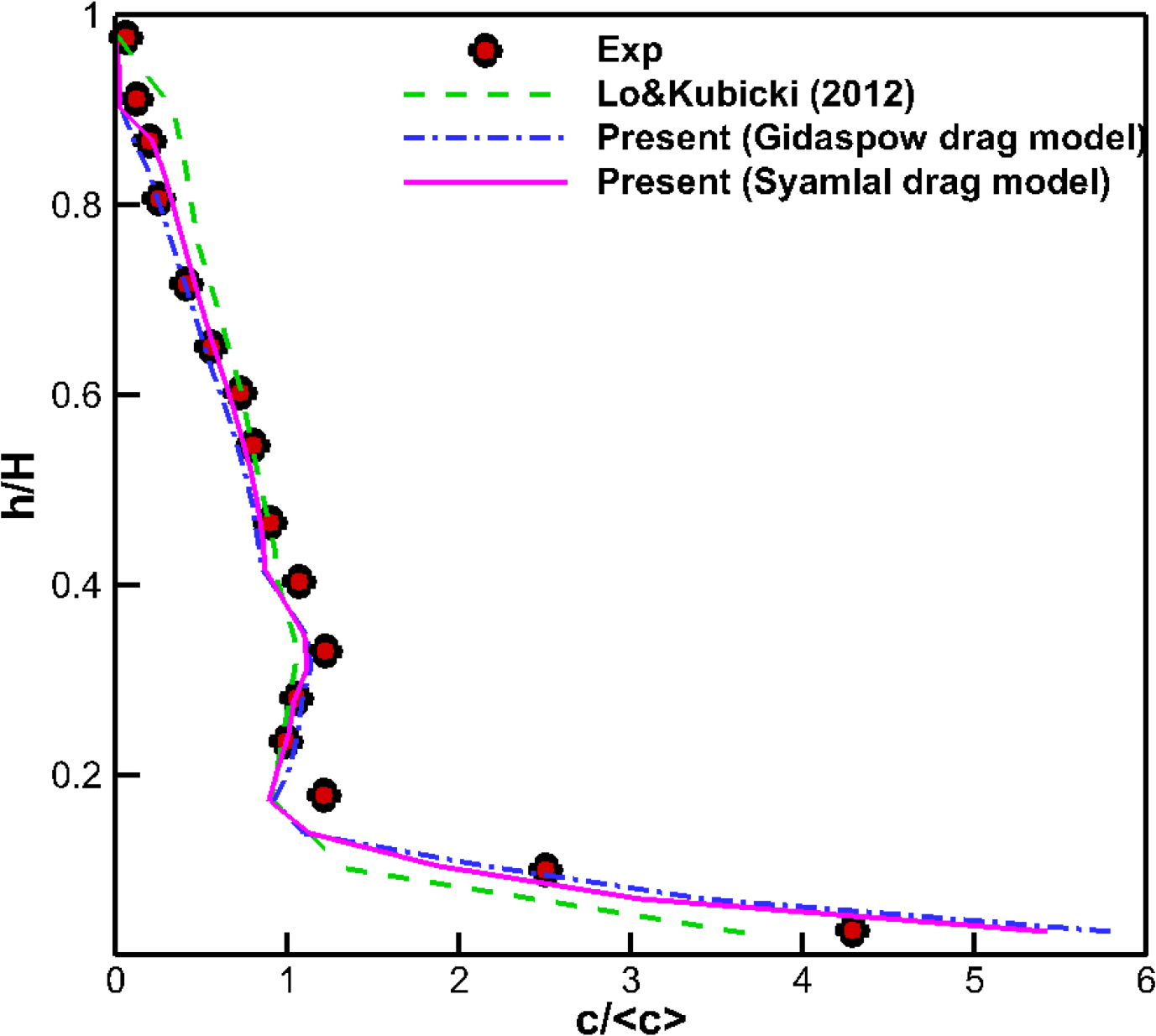
Simulation results for the interaction model tests are shown in Figs. 12–13. The results show that the lift model has less effect on the concentration distribution, whereas for the drag model, the concentration distribution with Syamlal and O’Brien’s drag model becomes closer to the experiment. This suggests that the drag coefficient calculated directly from flow field of the Syamlal-O’Brien drag model is more suitable for the prediction of concentration. In addition, the simulation results obtained in this study show that the concentration distribution is more similar to that of the experiment compared to the other CFD simulation, especially in the lower part (Kubicki and Lo, 2012).
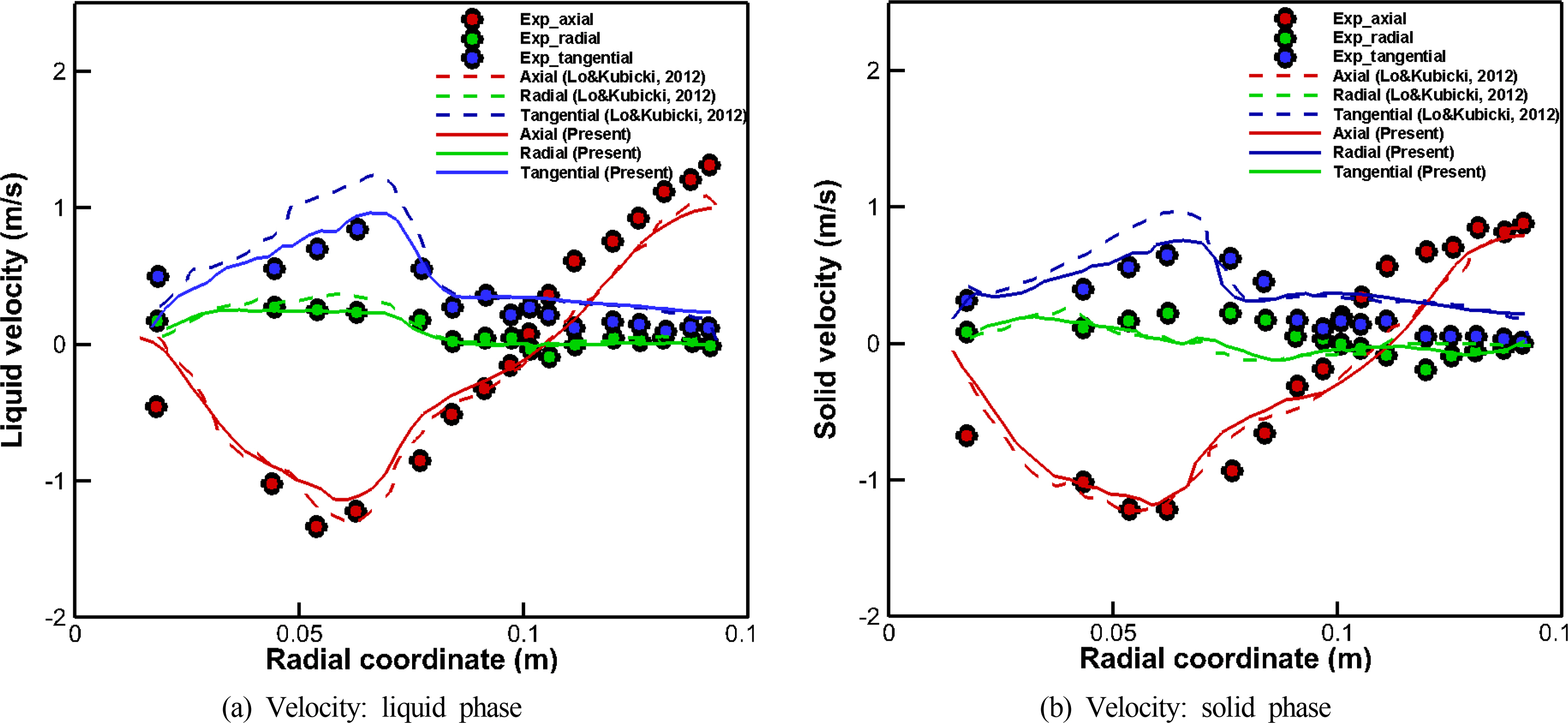
Finally, based on the Syamlal-O’Brien drag model, the three velocity components of each phase for the liquid and solid were compared with those from the experiments and other CFD simulations, as shown in Fig. 14. The overall trend of the velocity profiles shows that the simulation results and experiments are similar to each other. However, the tangential velocities for both liquid and solid phase have better agreement with the experiment than the other CFD simulation results. From these validation results, the Syamlal-O’Brien drag model was employed to simulate the multi-phase flow of a mud agitator in the next step.
3.3 Multi-phase Flow Simulation Around Mud Agitator
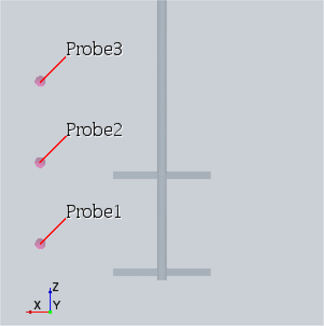
The mud agitator for the CFD simulation is a cube-shaped tank with a side length of 4 m. It contains a double-bladed impeller, which was modeled as shown in Fig. 15. The detailed dimensions of the mud agitator, including the inner 4-blade 45°-pitch impeller, are summarized in Table 2. The boundary conditions and grid system are almost the same as in the previous simulations, and about one million grid points were used. To account for the multi-phase mixing between the liquid mud and bulk (barite) in the mud tank, the liquid mud is assumed to be Newtonian fluid that has constant material properties. The detailed properties for each of the liquid and solid phases are specified in Fig. 15. To check the mixing process of the mud agitator, the concentration inside the mud tank was measured through probes located at three different heights, as shown in Fig. 16.
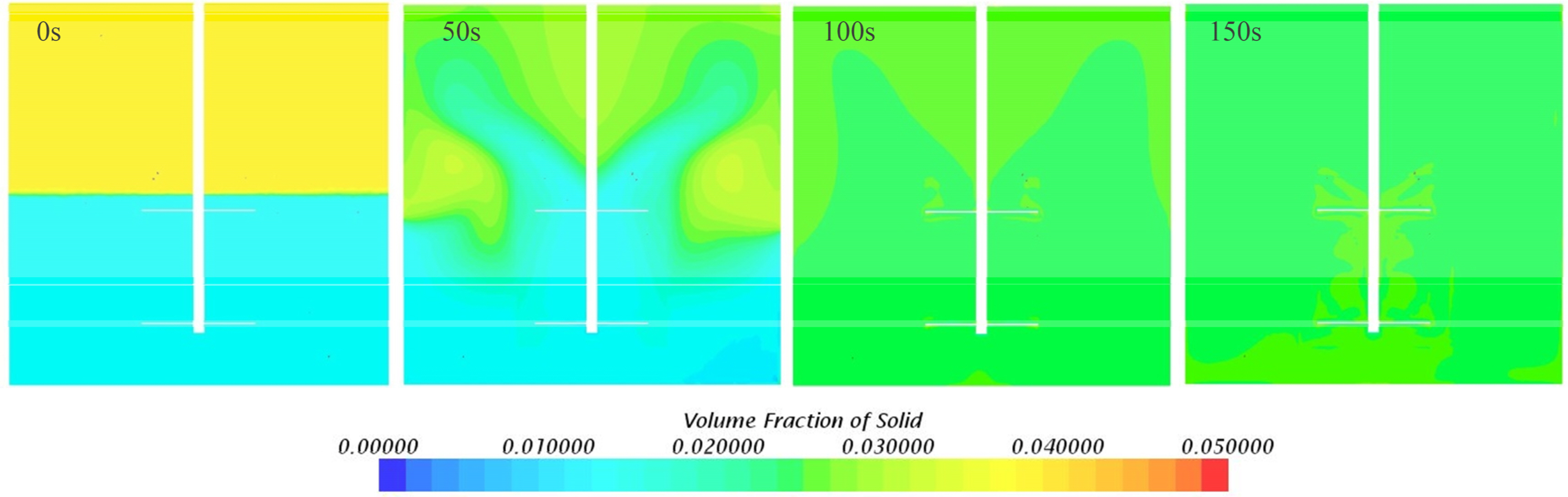
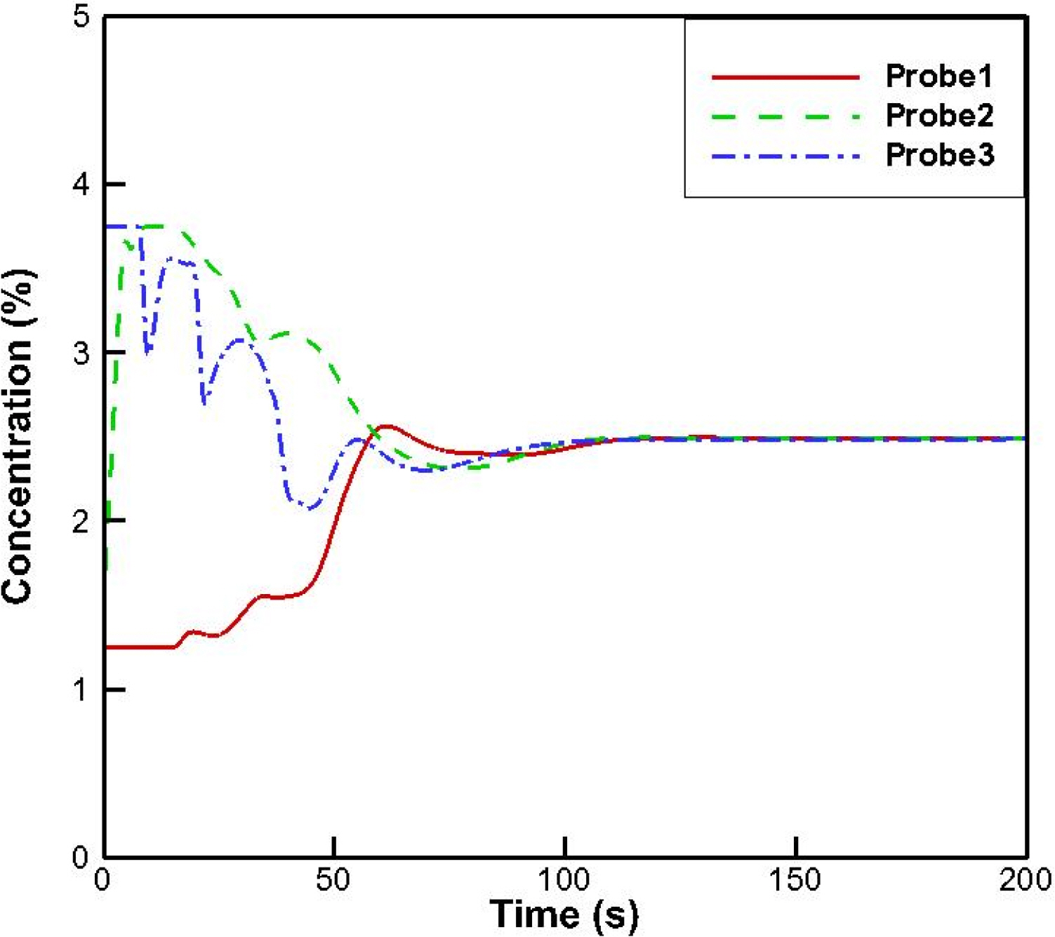
During actual operation, the role of the mud agitator is to maintain uniform density and viscosity of the pre-mixed mud. In this simulation, however, it is initially set to have a discontinuous concentration distribution as the initial distribution, as shown in in Fig. 16 (0 s). The average concentrations of the solid-phase at the higher and lower parts of the tank are 3.75% and 1.25%, respectively. As time goes by, as shown in Fig. 17, the concentration distribution of the solid phase in the space gradually becomes homogeneous and seems to be almost mixed after 100 s. In Fig. 18, it can be observed quantitatively that the time history of the concentration measured at 3 places converges to a constant value of about 2.5% after 100 s, and the mud becomes well mixed. The total torque acting on the two impellers after thoroughly mixing was calculated to be about 532 N·m, which can be seen to consume about 26.7% more power compared to mixing single-phase water.
4. Conclusions
In this study, the mixing performance of a mud agitator for offshore drilling was evaluated through a CFD simulation based on an Eulerian-Eulerian approach. For verification of the CFD tool, the velocity distribution for the vortical flow of single-phase water generated by an impeller inside a model-scale tank was compared with an experiment (Guida et al., 2009; Guida, 2010). Moreover, after alternately employing various turbulence models (STE, RKE, KW, RSM, and LES), the SKE showed more valid results with respect to the experiment and faster in computation. Thus, it was selected through comparison of the average velocity distribution during the mixing process.
Subsequently, a comparison of the multiphase interaction models was performed in the mixing problem for the liquid-solid multiphase flow. As a result, it was found that the Syamlal-O’Brien drag model, which directly calculates the drag coefficient, has better agreement with the experiment (Guida et al., 2009) than other CFD results (Kubicki and Lo, 2012) in the concentration distribution and velocity file during the mixing process. Using the verified simulation conditions, a liquid-solid multiphase flow simulation was then performed. In the simulation, it was observed that the solid concentration uniformly converged and mixed well in all places measured