


1. Introduction
In these days, countries around the world have been implementing increasingly stringent environmental regulations on ships. In particular, the International Maritime Organization (IMO) has enforced the regulation to reduce the maximum permitted sulfur content of the exhaust gas emitted from ships from 3.5% to 0.5% since January 1, 2020, and the Maritime Emission Protection Committee (MEPC) agreed to a minimum 50% reduction of the annual greenhouse gas emissions from the total ships by 2050 compared to the level of greenhouse gas emissions in 2008 (Jeong, 2019; Park, 2019; Ji and El-Halwagi, 2020). As a result, alternative energy sources, such as LNG and hydrogen, have begun to attract considerable attention. On the other hand, because LNG-powered ships still emit greenhouse gases (GHG), it is difficult to achieve the MEPC GHG reduction target, even if all the currently operated vessels are replaced with LNG-powered ships. Therefore, from a long-term perspective, hydrogen-powered ships are attracting increasing attention since hydrogen has similar advantages to LNG. Moreover, hydrogen-powered ships have low noise and vibration, a simple drive system, and no GHG emissions (Lee et al., 2019).
Like LNG, hydrogen needs to be kept in a cryogenic liquid state to maximize its transportation efficiency. Accordingly, it is necessary to develop technologies for a cargo handling system (CHS) and fuel gas supply system (FGSS) by considering insulation and boiling. Hence, methods for accurate analysis of the characteristics of cryogenic liquids are needed to determine the equipment-related specifications of these systems and develop safety standards.
In the analysis of the thermal flow in a pipe through which a cryogenic liquid flows, the physical phenomenon that needs to be considered is ŌĆśboilingŌĆÖ. When a cryogenic liquid flows through a pipe, boil-off gas (BOG) or vapor is generated due to the boiling phenomenon caused by heat transfer resulting from the temperature difference between the wall surface and the liquid. An increase in the amount of BOG causes changes pressure in the pipe leading to safety problems. Problems related to BOG generation while transporting cryogenic fluids need to be dealt with urgently before hydrogen-powered ships can be commercialized.
Experimental studies have been carried out to improve the heat transfer performance or investigate the impact of critical heat flux on the industrial equipment and systems in relation to the thermal performance of industrial equipment, such as boilers, nuclear reactors, and cryogenic fluid systems (Krepper et al., 2007). Bartolemei and Chanturiya (1967) proposed relationships between the fluid enthalpy, temperature, and void fraction based on the experimental results. Tolubinsky and Kostanchuck (1970) presented the relationships between the subcooling temperature, bubble departure diameter, and frequency derived from experiments.
In recent years, at the forefront of various engineering design areas, the analysis of fluid flow problems using computational fluid dynamics (CFD) has been gaining attention. Studies to elucidate the process of boiling have been conducted mainly in the field of nuclear engineering. Krepper et al. (2007) performed CFD analysis to compare the experimental values reported by Bartolemei and Chanturiya (1967) with the simulated values. Sontireddy and Hari (2016) compared the Rohsenow boiling model and the wall boiling model with the experiments reported by Bartolemei and Chanturiya. Gu et al. (2017) explained the boiling of subcooled liquids through the combination of several correlation equations using the wall boiling model.
In the present research, one of the experimental cases of Bartolemei and Chanturiya (1967) was implemented using the commercial software, STAR-CCM+ (ver. 15.02.007) to perform a CFD simulation of multiphase-thermal flow considering boiling in the pipes for the transport of cryogenic liquids. Comparative studies of the sensitivity and convergence between different combinations of parameters were performed by varying the coefficients used in the phase change models and grid size.
2. Subcooled Boiling Model
Subcooled boiling occurs when the liquid temperature is lower than the boiling point and the temperature of the wall surface is higher than the boiling point. This refers to a boiling phenomenon, in which bubbles are formed on the heated wall surface, detached from the wall, and absorbed into the liquid. The boiling phenomenon occurs at the initial point of wall boiling when the heat flux is transmitted from the wall, and it is observed in most flows in the pipes. On the other hand, saturated boiling refers to a boiling phenomenon that occurs when most of the liquid reaches the saturation temperature. It occurs when a liquid with the saturation temperature passes over the wall surface that has heat flux. A much larger amount of BOG is generated by saturated boiling than subcooled boiling, so the transportation efficiency is increased if the liquid is set up to maintain a subcooled state when flowing through a pipe.
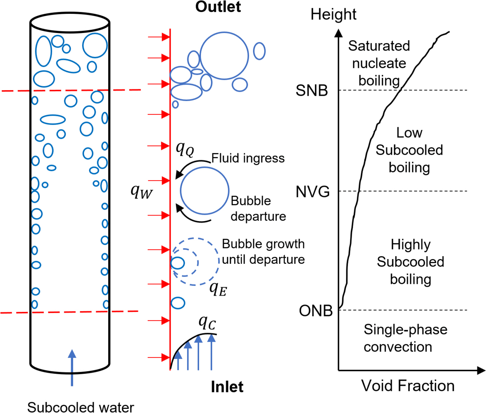
For example, Fig.1 shows a schematic view of applying the wall boiling model to the experiment reported by Bartolemei and Chanturiya (1967). If subcooled water flows through a pipe and contacts the pipe wall with heat flux, the heat flux is initially used only to increase the temperature of the liquid near the wall. Convection occurs in both the flow near the wall and the flow distant from the wall, resulting in a temperature layer. When the liquid near the wall passes through the onset of nucleate boiling (ONB) stage and reaches the saturation temperature, bubbles are formed in the liquid near the wall. As this vaporization process occurs, boiling occurs gradually. Moreover, as the liquid passes through the net vapor generation (NVG) point, bubbles formed on the wall reach the critical diameter and detach from the wall. Up to this point, some of the liquid detached from the wall is still in a subcooled state, and when the liquid passes through the saturated nucleate boiling (SNB) point, all the liquid in the pipe reaches the saturation temperature.
Approaches of the numerical simulation for multiphase flows using STAR-CCM+ are divided mainly into the volume-of-fluid (VOF) model, the Eulerian mixture model, and the Eulerian multiphase model. Among them, the VOF model calculates the volume fraction of each fluid in the analysis region using a momentum equation for two-phase flow, which are flows of two or more immiscible fluids. This model is applicable to jet flows, bubble flows, and free surface flows. The Eulerian mixture model is similar to the VOF model, but the Eulerian mixture model assumes that the phases can interpenetrate each other. Hence, this model is applied frequently to the problems of pipe flow or mixing flow. Lastly, in the Eulerian multiphase model, it is assumed that the laws of conservation of mass, momentum, and energy are applied to each phase individually with respect to two-phase flows consisting of phases that are treated as interpenetrating continua. Therefore, this model can be applied to several multiphase flow problems that are difficult to deal with using the other two models, but considerable computation time is needed. In this study, the numerical simulation results of the boiling phenomenon obtained by two different methods, the VOF model and the Eulerian multiphase model, were compared. The two specific models considered in this study were the Rohsenow boiling model among the VOF models and the wall boiling model among the Eulerian multiphase models.
2.1 Rohsenow Boiling Model
The Rohsenow boiling model is a relational expression for a model for nucleate boiling by natural convection and was presented experimentally by Rohsenow (1952). In this model, the heat flux transferred from the wall to the liquid is determined by Eq. (1).
where ╬╝l is the dynamic viscosity of the liquid phase; hlat is the latent heat of vaporization; g is the gravitational acceleration; Žül is the density of the liquid; Žüv is the density of the vapor; Žā is the surface tension coefficient at the liquid-vapor interface; CPl is the specific heat of the liquid phase; Tw is the temperature of the wall; Tsat is the saturation temperature; Cqw is an empirical coefficient varying with the liquid-surface combination; Prl is the Prandtl number of the liquid; np is the Prandtl number exponent that depends on the surface-liquid combination.
2.2 Wall Boiling Model
The wall boiling model is the nucleate boiling model proposed by Kurul and Podowski (1991), as shown in Fig. 1. The heat flux transferred from the wall to the liquid, , is divided into three components as follows:
where qC represents convective heat flux, which refers to the contribution of the heat flux transferred from the wall to the convection of the liquid, and is defined by Eq. (4).
where hC indicates the single-phase heat transfer coefficient; Tl is the average liquid temperature; Ab is a coefficient that depends on the bubble departure diameter and the nucleation site density; K is an empirical constant; NW is the nucleation site density; dW is the bubble departure diameter; Jasub is the subcooled Jacob number; ŌłåTsub =Tsat ŌłÆTl represents the subcooling temperature of the liquid; hlat is the latent heat of evaporation.
qE indicates the evaporation heat flux. It refers to the contribution of the heat flux transferred from the wall to the boiling of the liquid, and is expressed using Eq. (8).
where Vd indicates the volume of vapor bubbles for the bubble departure diameter, and f represents the bubble departure frequency defined by Cole (1960).
Finally, qQ is the quenching heat flux, which refers to the average heat flux transferred to the liquid when the liquid occupies an empty space immediately after bubble departure, and it is defined using Eq. (11).
where kl indicates thermal conductivity; ╬╗l indicates the diffusivity of the liquid; Žä is the periodic time of bubble departure.
In deriving the accurate results from the wall boiling model applied to the analysis of various boiling problems, the most dominant parameters are, NW, dW and f. As these parameters vary according to diverse factors, they are generally derived empirically through experiments, and the correlations between these parameters have been studied widely (Kurul, 1990; Alglart, 1993; Alglart and Nylund, 1996; Tu and Yeoh, 2002; Lee et al., 2002; Koncar et al., 2004; Krepper et al., 2007; Chen and Cheng, 2009; Krepper and Rzehak, 2011; Nemitallah et al., 2015; Gu et al., 2017). Previous studies have been confined mostly to selecting the optimal combination of submodels (nucleation site density and bubble departure diameter models), which is suitable only for a specific pressure section of a pipe. Gu et al. (2017) compared five combinations of submodels using ANSYS Fluent, a commercial analysis program. Compared to ANSYS Fluent, STAR-CCM+ used in this study has limitations in that it does not include the model proposed by Unal (1976) among the bubble departure diameter models. On the other hand, as some combinations were omitted from the comparison in Gu et al. (2017), it was considered necessary to conduct a comparative study using the combinations provided by STAR-CCM+. Therefore, in the present study, an overview of the and models provided by STAR-CCM+ were presented, and a parametric study on the combination of NW and dW models and the minimum bubble departure diameter was investigated.
2.2.1 Nucleate site density, NW
The empirical equation for presented by Lemmert and Chawla (1977) is as follows (LC model):
where C and n are coefficients determined based on experimental data; they were estimated to be 210 and 1.805, respectively, in Kurul and Podowski (1991).
On the other hand, an empirical equation for NW proposed by Kocamustafaogullari and Ishii (1983) is as follows (KI model):
where ŌłåTe represents the effective superheat, and S is the suppression factor.
2.2.2 Bubble departure diameter, dW
The general correlation for dW proposed by Tolubinsky-Kostanchuk (1970) is as follows (TK model):
As shown in Eq. (17), the bubble diameter is limited to 1.4 mm or less in the TK empirical model.
On the other hand, Kocamustafaogullari and Ishii (1983) presented the correlation for dW as follows (KI model):
where ŽĢ represents the contact angle of bubbles, and ŽĢ was set to be 80┬░ in Rogers and Li (1994).
3. Numerical Simulation
3.1 Setting Up the Problem of Flow Boiling in a Tube
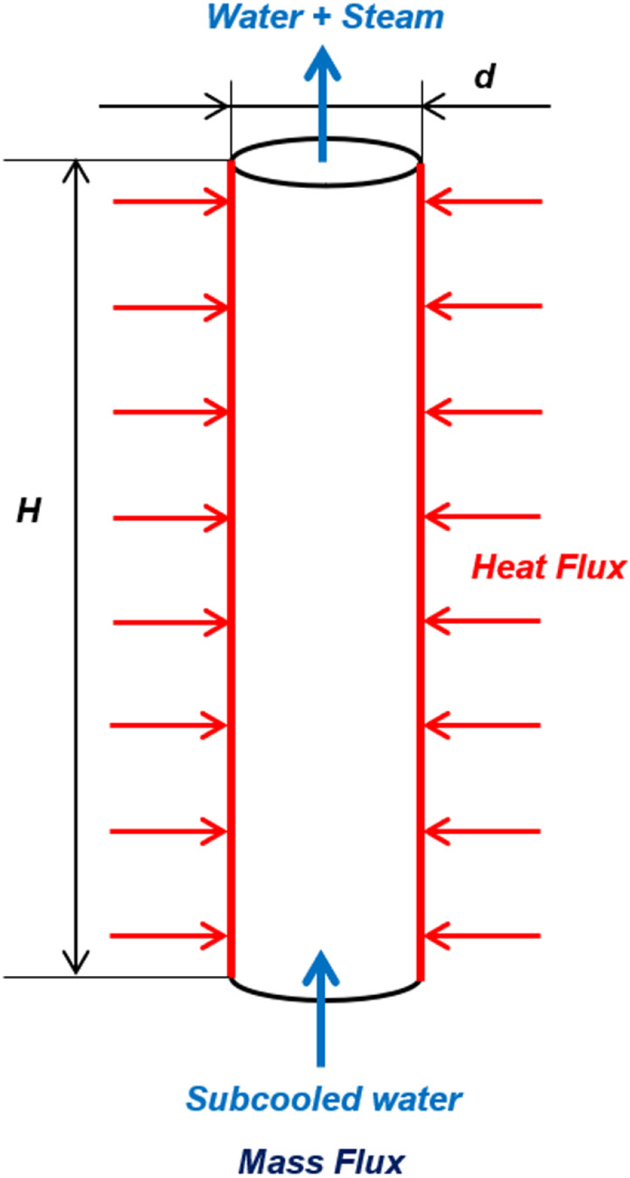
The accuracy of the boiling model was verified by numerical simulations referring to the experiment conducted by Bartolemei and Chanturiya (1967). As shown in Fig. 2, in the experiment of Bartolemei and Chanturiya (1967), subcooled water with a temperature of 470.63K was induced to flow at a mass flow rate of 900kg/m2┬Ęs into a vertical tube made of stainless 1Cr18Ni9Ti steel with a height (H ) of 2.0m and a diameter (d) of 15.4mm. A constant heat flux of 570 kW/m2 was applied to the surrounding wall to induce a phase change of the water into vapor, and the temperature and vapor content according to the flow enthalpy were measured. At this time, the initial pressure inside the tube was set to 45 bar (= 45 ├Ś 105 Pa).
The conditions and configuration of the numerical simulation were set to be as similar as possible to those of the experiment, as shown in Fig. 3. As reported by Wang and Yao (2016), there were only slight differences between the analysis results of two-dimensional and three-dimensional simulations of multiphase flows in a cylindrical-shaped tube. Hence, two-dimensional simulations were carried out by applying the axis of symmetry to reduce the computation time. At the inlet, the vertical length of the inlet region (Linlet) was set to 0.5m to allow subcooled water to achieve fully developed flow. At the outlet, the vertical length of the outlet region (Loutlet) was also set to 0.1m to allow the flow to exit smoothly. Furthermore, by applying axial symmetry, only one wall in Fig. 3 was heated with the heat flux level observed in the experiment. Adiabatic conditions were set for other walls except for the heated section. The simulations were conducted by assuming a steady state based on Sontireddy and HariŌĆÖs (2016) results, who reported no significant differences in the simulation results between the steady and unsteady states.
3.2 Simulation Results
Regarding the subcooled boiling phenomenon in a boiling tube, the void fraction according to the height was calculated by applying the Rohsenow boiling model and the wall boiling model. The simulations were compared with the experimental results (Bartolemei and Chanturiya, 1967). In the case of the wall boiling model, as summarized in Table 1, the simulation was performed using the combinations of important parameters, such as the nucleation site density and the bubble departure diameter models. After a comparative analysis of the simulated values obtained through simulation, the Kocamustafaogullari-Ishii(KI) model of the nucleation site density model was applied as the final selected condition. Thereafter, for cases to which the KI model was applied for the bubble departure diameter model, after evaluating the grid convergence, research was carried out by varying the minimum diameter of vapor bubbles.
3.2.1 Comparison between different boiling models
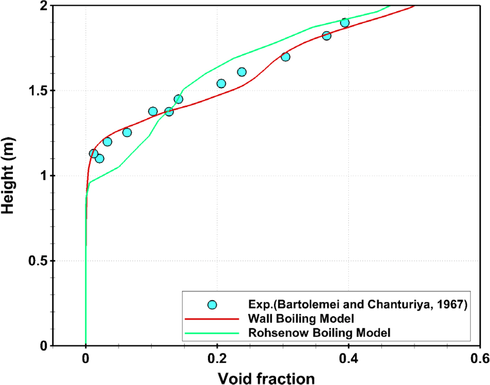
Fig. 4 shows the void fraction distribution obtained by applying two different boiling models. In the Rohsenow boiling model, the comparison between simulated and experimental values showed that the initial bubble formation proceeded faster. In the wall boiling model, however, the simulation results from initial bubble formation to the bubble growth process were in relatively good agreement with the experimental values. This difference was because the Rohsenow boiling model does not appropriately reflect the boiling process by forced convection (Domalapally et al., 2012). Boiling by forced convection occurs due to the forced motion of a fluid. Therefore, to consider this phenomenon in future studies, it is necessary to make a comparison by applying the boiling model proposed by Bergles and Rohsenow (1964). On the other hand, a comparison of the void fraction values near the outlet showed that both models yielded void fractions that approximated the experimental values very closely. On the other hand, as summarized in Table 2, a comparison of the total solver elapsed time showed that the wall boiling model took approximately two times longer calculation time than the Rohsenow boiling model. Therefore, the wall boiling model appears to be more suitable for analyzing subcooled boiling problems, including the bubble formation and growth processes near the wall but required two times longer computation time.
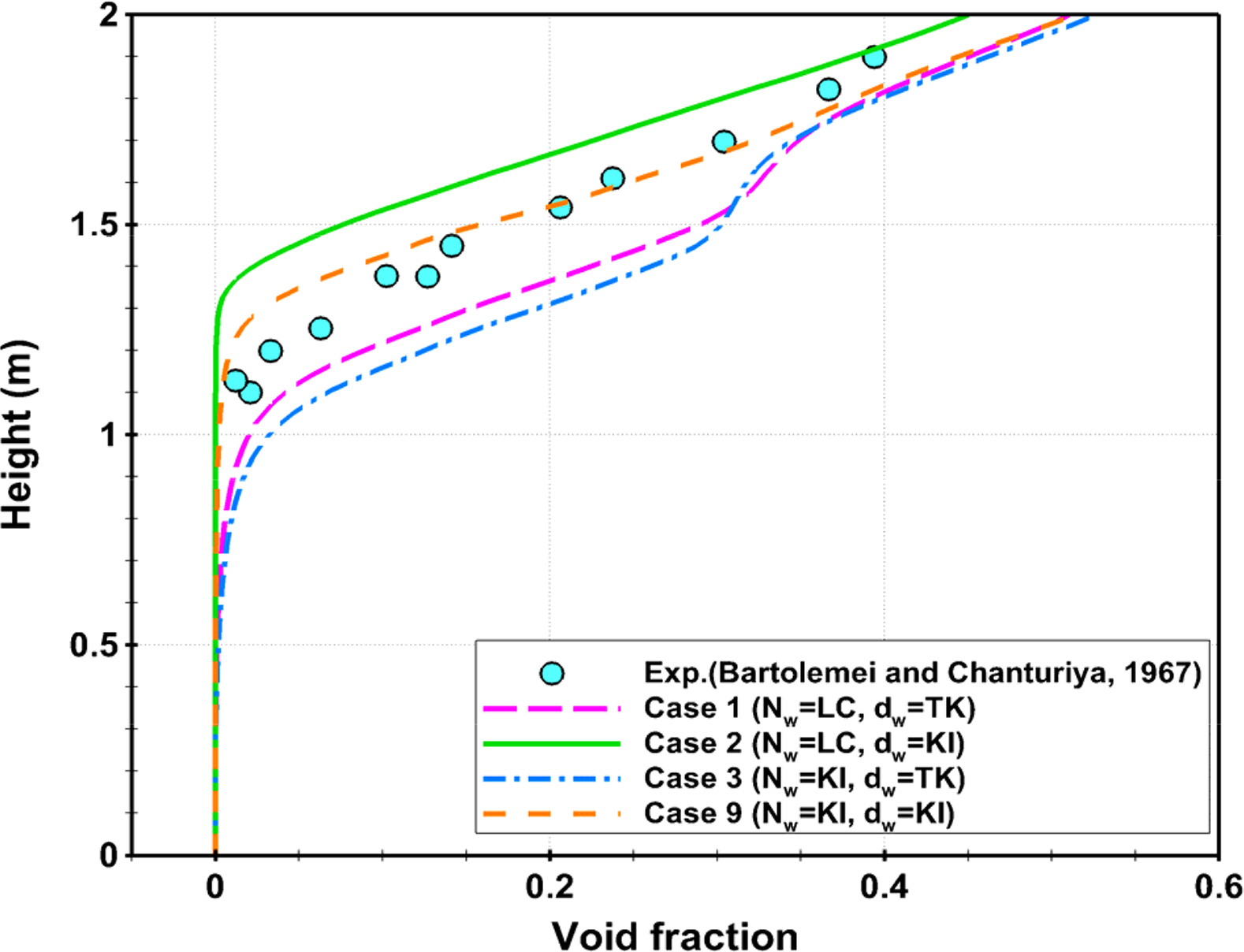
3.2.2 Comparison of the simulation results by different combinations of nucleation site density and bubble departure diameter models (Cases 1-3 & 9)
For Cases 1-3 and 9 in Table 1, Fig. 5 shows the void fraction distribution according to the height. Comparative analysis is needed because the accuracy of the wall boiling model varies according to the combination of the nucleation site density model and the bubble departure diameter model. An examination of the void fraction distribution obtained by each model combination showed that the changes depending on the bubble departure diameter model were more pronounced than those depending on the nucleation site density model. For this reason, the results obtained by applying the KI model as the bubble departure diameter model were closer to the experimental values. On the other hand, the comparison of Case 2 with case 9 showed that Case 9, in which the KI model was applied as the nucleation site density model, approximated more closely the range of the void fraction distributions measured in the experiment. Based on these results, for the cases where the KI model was applied for both the nucleation site density model and the bubble departure diameter model, the grid convergence test and the sensitivity test were conducted to evaluate the grid convergence and sensitivity according to the minimum bubble diameter. Sections 3.2.3 and 3.2.4 present the methods and results of the grid convergence test and the sensitivity test, respectively.
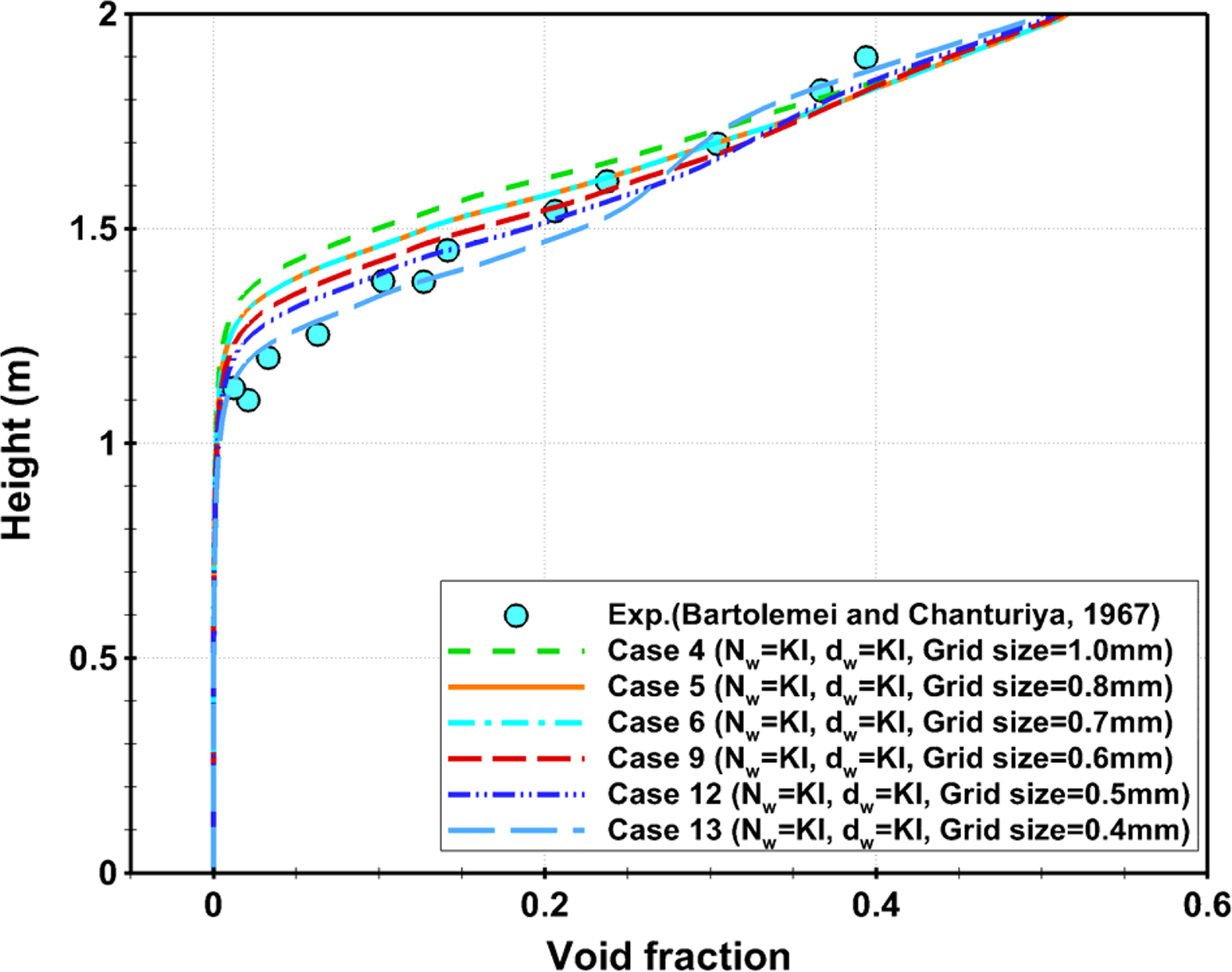
3.2.3 Grid convergence test (Cases 4ŌĆō6, 9, 12 & 13)
Fig. 6 shows the void fraction distribution among the results obtained by the grid convergence test for cases where the KI model was applied in both the nucleation site density model and the bubble departure diameter model. As the grid size became smaller, there was a larger difference between the void fraction distribution in the section of H = 1.1ŌĆō1.7 m (the ONB-SNB section), where the initial bubbles started to be generated on the wall, and the results closely approximated the experimental results. At the outlet region, however, there was no significant difference in the void fraction according to the grid system.
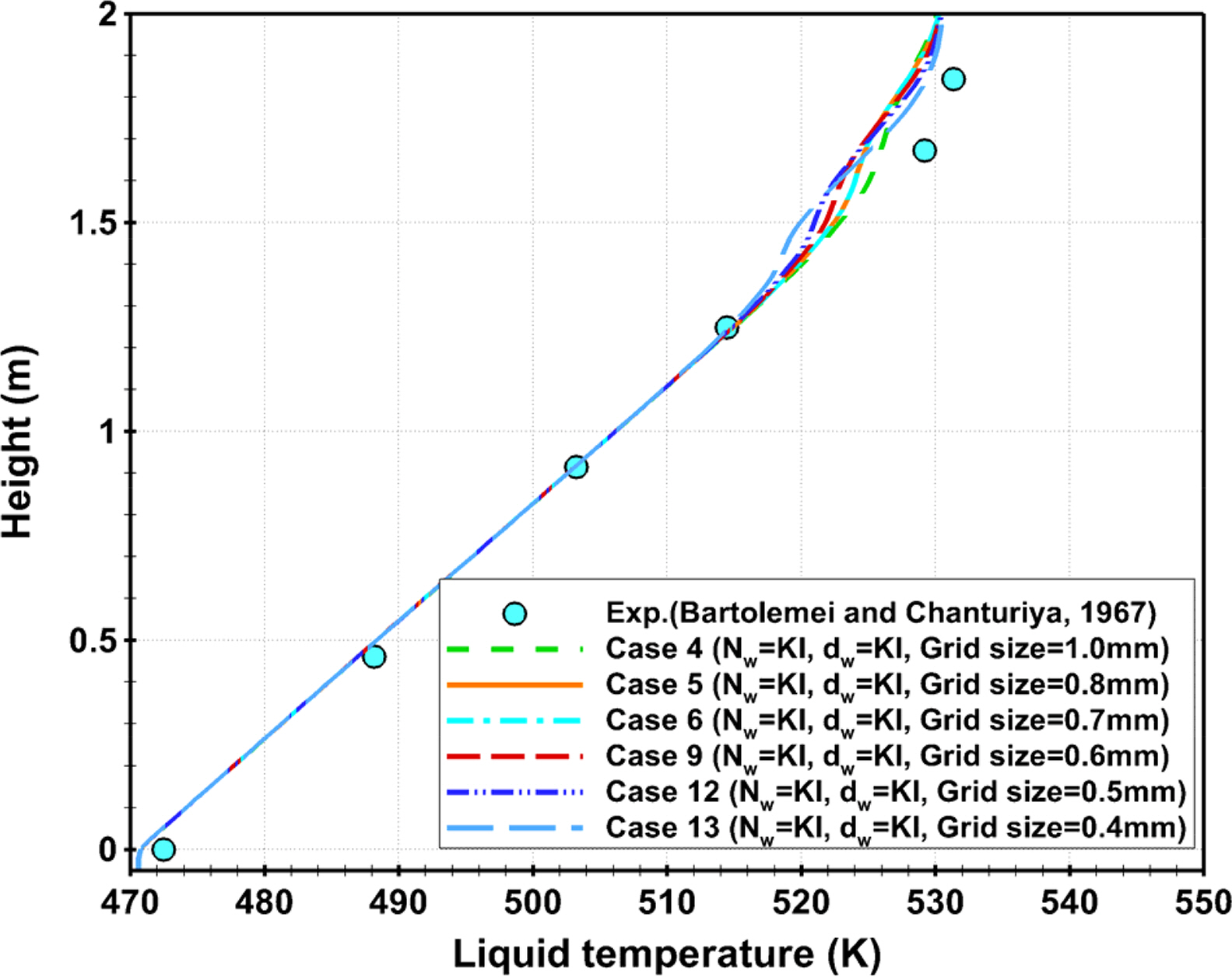
Fig. 7 presents the temperature distribution of the liquid according to the grid system along the central axis of symmetry in the pipe. Looking into the result, the impact of the grid size was found to be mostly insignificant in the overall sections from the inlet region to the onset of nucleate boiling (ONB) section. However, in the net vapor generation-saturated nucleate boiling (NVG-SNB) section (H Ōēł 1.3ŌĆō1.7 m), where the ratio of vapor in the internal liquid becomes relatively higher, large differences according to the grid size were observed. This is believed to be related to the grid resolution, which indicates the degree of ability to represent the mixture of the generated vapor and liquid numerically. On the other hand, in the SNB section (H Ōēł 1.7ŌĆō2.0 m), where saturation boiling is dominant, there was a slight difference between the simulated and experimental values regardless of the grid resolution. This disparity was attributed to the increased outlet region for a stable numerical calculation and the constant temperature for the added outlet region. Another cause is believed to be differences due to the combination of the nucleate site density model and bubble departure diameter model. Gu et al. (2017) applied the LC model to the nucleate site density and the KI model to the bubble departure diameter. They reported that the numerical results for the liquid temperature distribution in the same section (H Ōēł 1.7ŌĆō2.0 m) showed good agreement with the experimental results. On the other hand, a comparison of the void fraction distribution showed large differences. These results suggest that when multiphase-thermal flow in a pipe is simulated, the model combination selected may vary depending on which physical quantities are used as the basis for analysis. Therefore, it is important to apply the optimal boiling model through the combination of submodels and parametric studies.
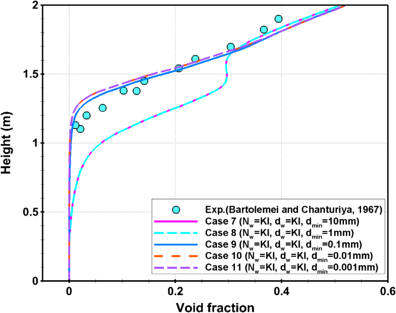
3.2.4 Relationship between the minimum bubble departure diameter and grid size (Cases 7ŌĆō11)
Section 3.2.3 showed differences in the growth process of initial bubbles according to the grid size. This section analyzed the relationship between the grid size and the minimum bubble departure diameter. Fig. 8 presents the void fraction distribution obtained by fixing the grid size and varying the minimum diameter of bubbles. The void fraction distribution could be clearly distinguished based on the minimum bubble departure diameter of 1mm. In Cases 7ŌĆō11, the grid size is 0.6 mm, and it can be seen that the accuracy of the boiling model may be decreased when the minimum bubble departure diameter is 1 mm or 10 mm, which is larger than the grid size. On the other hand, all the results tended to converge when the minimum bubble departure diameter was smaller than the grid size.
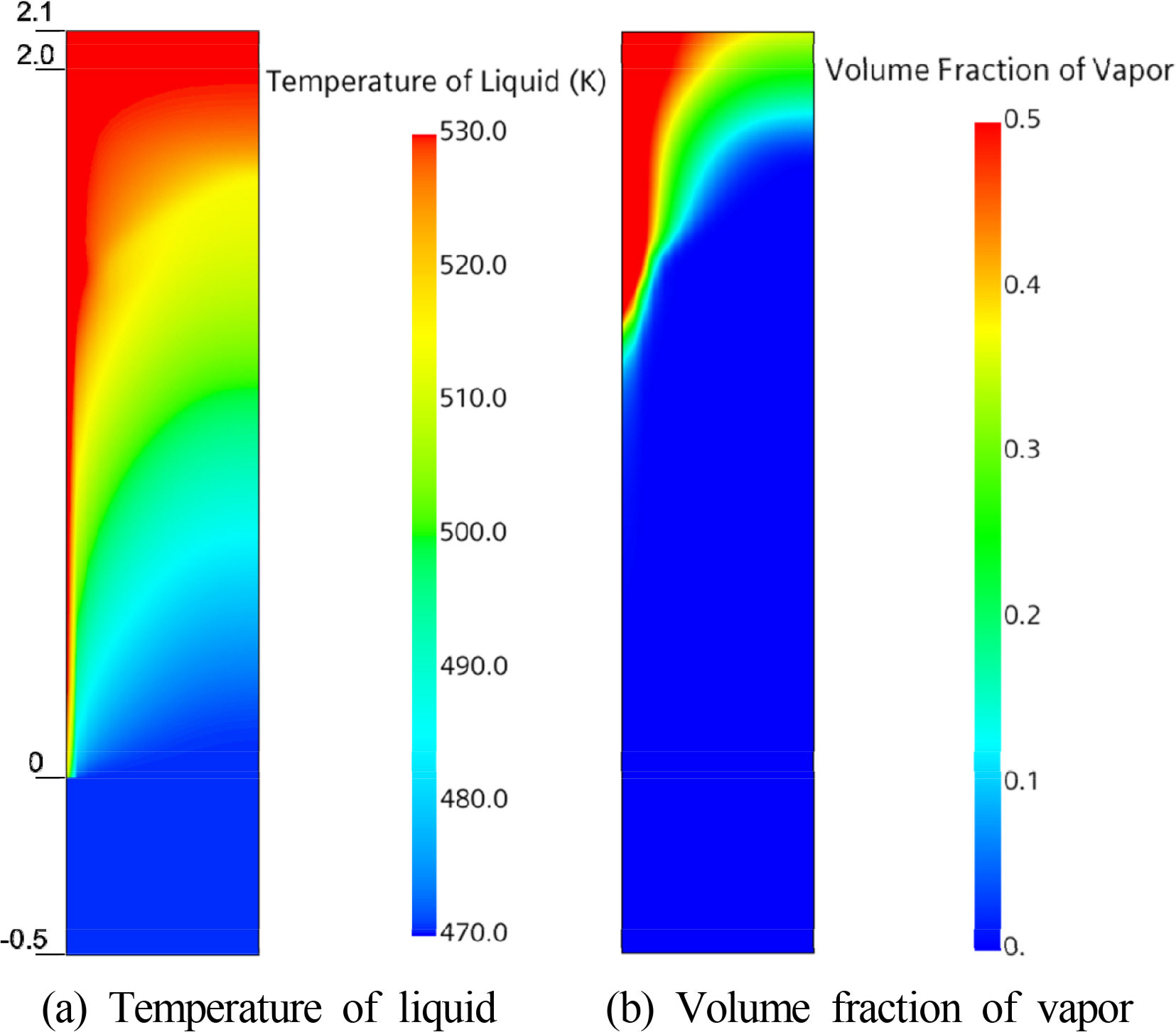
3.2.5 Results of subcooled boiling (Case 9)
Fig. 9 presents the temperature distribution of the liquid in the pipe and the volume fraction of vapor obtained by numerical simulation for Case 9. The left wall of the tube is heated, and the central axis of symmetry is located on the right. The temperature distribution of the liquid suggests that as subcooled water flows into the heated pipe, the water temperature near the wall increases, and the temperature distribution of the flow in the entire pipe changes with increasing height. In addition, the distribution of the volume fraction of vapor shows the mechanism through which as the temperature of the liquid near the wall becomes higher than the saturation temperature; the liquid changes into a vapor, and the liquid and vapor are mixed in the pipe.
4. Conclusion
To simulate multiphase-thermal flow in a pipe, including phase change, the applicability of the VOF model and Eulerian multiphase model, which are numerical models representing the phase change in the Eulerian-Eulerian framework, was verified and investigated. This paper reviewed the major aspects of the heat flux transferred from the wall to the liquid in relation to the Rohsenow boiling model among VOF boiling models and the wall boiling model among Eulerian multiphase models. A comparison of the Rohsenow boiling model and wall boiling model showed that the Rohsenow boiling model does not appropriately represent the initial bubble generation process, but it was closer to the experiment in the case of fully developed flow with a high percentage of vapor. Furthermore, the Rohsenow boiling model required smaller computing power than the wall boiling model. On the other hand, comparative analysis of different combinations of the nucleation site density and bubble departure diameter models used in the wall boiling model showed that the dependence on the bubble departure diameter model was more significant than the dependence on the nucleation site density model. In the grid convergence test for the selected combination of models, the ONB point, which is the location where the initial bubble formation starts at the heated surface, varies according to the grid size. This result highlights the necessity for caution in selecting the grid size. In conclusion, the results of the sensitivity test suggested that the grid size needs to be larger than the minimum bubble departure diameter to establish accurate predictions of the ONB location and a realistic representation of the bubble development process. The results of this research can be used in analyses to identify the dynamic characteristics of pipes constituting the cargo handling system (CHS) of transport ships handling cryogenic liquefied gases, such as LNG and liquid hydrogen, or pipes comprising the fuel gas supply system (FGSS) of propulsion ships as well as to determine the specifications of related systems. Multiphase-thermal flow analysis in various shaped cryogenic pipes, including insulation, will be performed in a follow-up study. Furthermore, this study will be applied to high accuracy analysis for establishing safety standards for related systems.