A Study on the High-Order Spectral Model Capability to Simulate a Fully Developed Nonlinear Sea States
Article information

Abstract
Modeling a nonlinear ocean wave is one of the primary concerns in ocean engineering and naval architecture to perform an accurate numerical study of wave-structure interactions. The high-order spectral (HOS) method, which can simulate nonlinear waves accurately and efficiently, was investigated to see its capability for nonlinear wave generation. An open-source (distributed under the terms of GPLv3) project named “HOS-ocean” was used in the present study. A parametric study on the “HOS-ocean” was performed with three-hour simulations of long-crested ocean waves. The considered sea conditions ranged from sea state 3 to sea state 7. One hundred simulations with fixed computational parameters but different random seeds were conducted to obtain representative results. The influences of HOS computational parameters were investigated using spectral analysis and the distribution of wave crests. The probability distributions of the wave crest were compared with the Rayleigh (first-order), Forristall (second-order), and Huang (empirical formula) distributions. The results verified that the HOS method could simulate the nonlinearity of ocean waves. A set of HOS computational parameters was suggested for the long-crested irregular wave simulation in sea states 3 to 7.
1. Introduction
The performance analysis of an offshore structure operating in the ocean is commonly requested to verify its survivability and operability over its expected design life. The most common way is to conduct an experimental campaign on the offshore platform in the wave basin. On the other hand, it is limited because of the scale effect, difficulty of measurement and modeling, cost, and the limitation of the experimental facility. Numerical analysis can be an alternative to an experiment because it can compensate for the experimental limitations. Nevertheless, it suffers from computational mesh modeling, numerical convergence, and a choice of numerical methods to simplify physical phenomena.
In both experiments and numerical simulations, the quality of ocean waves is the critical factor in modeling a realistic sea state. Therefore, the generated irregular waves experimentally and numerically should be qualified with the target sea state. In those applications, the irregular waves were qualified by comparing the sea spectrum, the significant wave height, and the peak wave period with the target sea state. On the other hand, considering the design of offshore structure dealing with extreme events, such as wave impact, air gap impact, and green water phenomena, the qualification of a local wave elevation, e.g., wave crest, becomes important and prevail nowadays. The measured wave elevation gives a wave crest probability distribution of single realization (PDSR). The PDSR is a probability distribution of the wave crest from one wave realization of a three-hour typical storm duration. The wave time signal in the experiment and numerical simulation with the limited number of irregular waves and different random seeds gives different wave crest PDSR curves. Hence, the PDSR curve made from a random seed can differ. Therefore, it is difficult to confirm the quality of the wave crest PDSR. Numerous wave realizations can be used to obtain the wave crest probability distribution of ensemble realization (PDER), which is a probability distribution of the wave crest from many three-hour realizations.
The obtained distribution of wave crest can be compared with the reference distributions. Longuet-Higgns (1952) reported the wave crest distribution of linear waves follows the Rayleigh distribution with assumptions of the Gaussian distribution and the narrow-band spectrum. On the other hand, the Rayleigh distribution underestimates the height of the wave crest when the sea states become severe, which can lead to a wrong design. Forristall (2000) suggested the wave crest distribution based on the second-order theory, which gives better results than the Rayleigh distribution. Later, Huang and Zhang (2018) suggested the semi-empirical formula of PDSR (mean and 99% upper bound and 99% lower bound) and PDER from the numerical wave simulation results of 305 sea states. The idea of Huang and Zhang (2018) was to qualify the PDSR with a single wave realization by comparing the distribution of wave crest probability of occurrence (POE) in the range of bounds of wave crest PDER. They compared the PDER between 100 realizations and 1000 realizations: the wave crest PDER showed a difference of −3% to +4% at the POE level of 10−4 and a −6% to +7% difference at the POE level of 10−5.
The irregular waves based on the superposition of linear waves are insufficient to model realistic ocean waves. Goda (1983) reported that the secondary peak due to the interaction of waves and nonlinearities is significant in ocean waves. Therefore, considering the nonlinearity is vital for the qualified local wave elevation. Tick (1963) and Hamada (1965) suggested the second-order irregular wave models. They reported that the second-order effect might not be enough to describe a higher-order interaction between wave components. The high-order spectral (HOS) method is a nonlinear wave generation method extending up to an arbitrary order (West et al., 1987; Dommermuth and Yue, 1987). One of the main strengths of HOS is that the derivatives that appear in nonlinear free surface boundary conditions can be treated in the frequency domain. Therefore, the fast Fourier transform (FFT) can be used in the numerical simulation, which makes the HOS method more efficient than the other numerical methods. The open-source project, called HOS-ocean, which models the open ocean by the HOS method, has been published (Ducrozet et al., 2007; Bonnefoy et al., 2009; Ducrozet et al., 2016). Moreover, they apply the HOS method for the numerical wave tank, which is also published as HOS-NWT (Ducrozet et al., 2012). The nonlinear irregular waves generated from the HOS method have been used to simulate the nonlinear waves in computational fluid dynamics (CFD) (Choi et al., 2018; Lu et al., 2022). Furthermore, those numerical tools have been used to simulate the wave-structure interaction problem (Li et al., 2019; Choi, 2019; Xiao et al., 2019). In addition, there was an attempt to define the standard protocol for irregular wave generation because it is used widely in industry and academia (Bouscasse et al., 2021).
Most academic research on applying the HOS model and CFD is limited to the extreme sea state. A parametric study of the HOS model for a wide range of sea conditions has not been conducted. In this context, this reports the results of a parametric study on the HOS method. As a parametric study, one hundred long-crested irregular wave simulations with different random seeds were performed for each sea state and selected HOS parameters for three hours. The present paper performed a stochastic analysis and analyzed the wave spectrum and wave crest height distribution by comparing them with references.
2. Numerical Wave Model
2.1 High Order Spectral Method
The open ocean is modeled with the rectangular computational domain with a length L in the x direction and a depth h in z direction. The sea bottom was assumed to be flat. The mean free surface was located at z = 0, and the z-axis was orienting upward. The perfect fluid and irrotational flow were assumed to introduce the velocity potential Φ. The velocity potential satisfied the Laplace’s equation in the fluid domain D as given in Eq. (1). The impermissible condition given in Eq. (2) was imposed on the sea bottom at z =− h. The periodic boundary condition shown in Eq. (3) is imposed at the lateral boundary.
On the free surface z = η(x,t), two free surface boundary conditions were imposed. The dynamic and kinematic free surface boundary conditions are given in Eqs. (4) and (5), respectively.
Φ̃(x;t)= Φ(x,z = η(x);t) is the free surface velocity potential, and w(x)= ∂Φ/∂z is the vertical velocity at the free surface z = η(x,t). The periodic boundary condition enables the free surface velocity potential and wave elevations with modal functions to be expressed as Eqs. (6) and (7).
The triangular system, which can be solved explicitly, can be obtained by expanding with respect to the order. The initialization of wave fields for the simulation is taken from the spectrum of irregular waves. The modal amplitudes of the wave elevation and free surface potential are taken as
3. Numerical Set-Up
3.1 Wave Condition
The wave conditions used in this study were taken from the sea state code suggested by World Meteorological Organization (WMO) (Lee and Bales, 1984; Lewis, 1989) to use representative wave conditions. Table 1 lists the wave conditions for each sea state code. In the present study, five wave conditions from sea state 3 to sea state 7, colored in Table 1, were considered, and the selected range corresponds to 90% of the annual sea state occurrence.
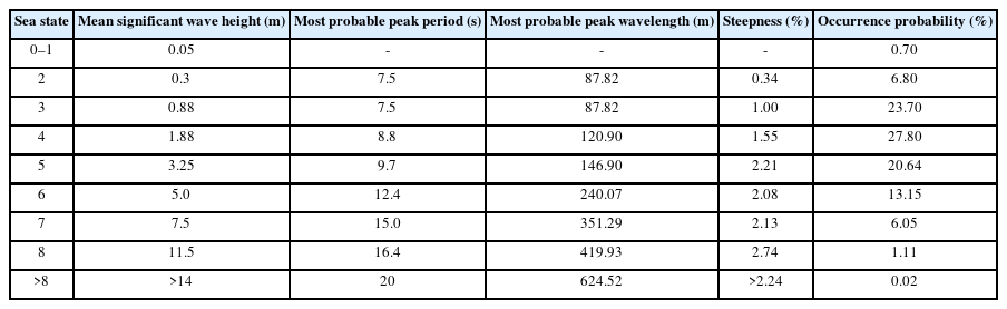
Annual sea state occurrences and wave parameters with respect to the sea states
A modified two-parameter Pierson-Moskowitz (P-M) spectrum is applied to describe the wave spectrum in a frequency domain (Kim, 2008) as expressed in Eq. (11). Here, ωp = 2π/Tp is the peak angular frequency, and Hs is the significant wave height of each sea state. Fig. 1 presents the considered wave spectra for different sea states.

Wave spectra for different sea states
3.2 HOS Computational Setup and Computational Parameters
The HOS fluid domain had a dimension of Lx = 15λp in the horizontal direction, and the deep water condition was assumed. Two computational parameters in the HOS method are important. The first was the order of nonlinearity, e.g., HOS order (M), and the second was the number of HOS modes (Nx ) corresponding to the number of spatial discretizations. Four HOS orders and three levels of HOS modes were adopted, as summarized in Table 2. Each HOS simulation was conducted for the three-hours, and 100 simulations with different random seeds were performed for each simulation setup. The HOS waves were measured at Lx = 5λp. For example, Fig. 2 shows a HOS wave time series of sea state 7 with the HOS order M = 4 and the HOS modes Nx = 512.
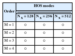
Considered HOS orders and the number of HOS modes
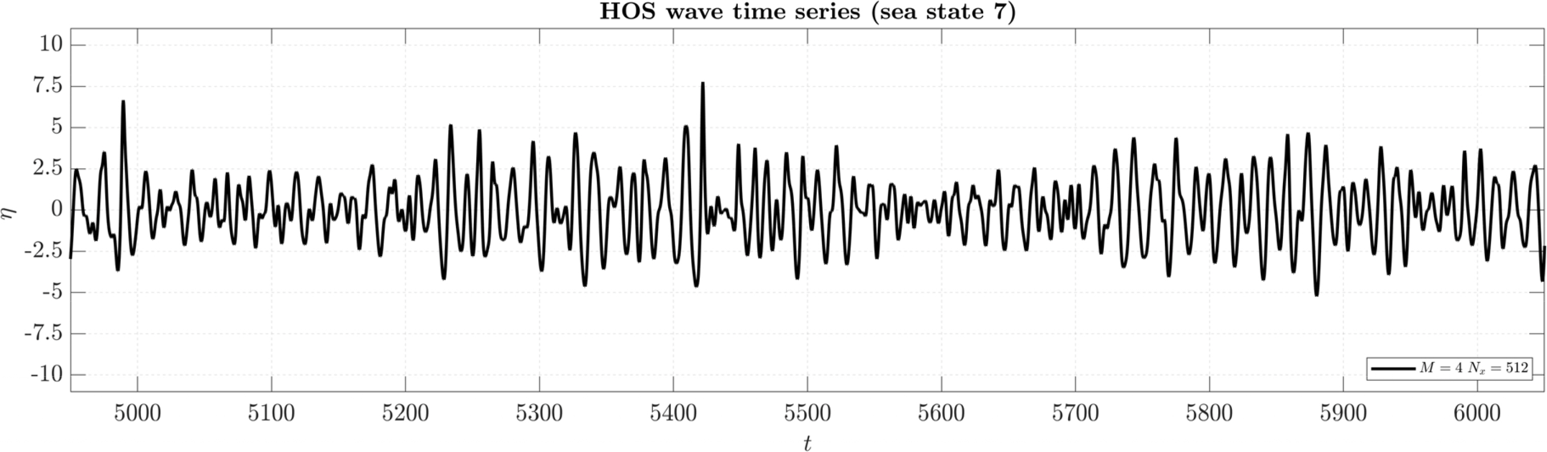
Example of the HOS wave time series (Nx = 512, M = 4)
4. Results and Discussions
4.1 Spectral Analysis
The wave spectrum was obtained from the wave elevation time series using Welch’s overlapped segment averaging estimator (Welch, 1967), where the window interval was approximately 15Tp. The averaged wave spectrum can be taken from 100 wave spectra and compared with the target wave spectrum. Fig. 3 gives an example of normalized wave spectra of sea state 7. The solid black line is a reference wave spectrum, and each colored marked lines are the wave spectrum with different combinations of HOS parameters. The wave spectra with HOS modes Nx = 128 clearly showed an overestimated spectrum compared to the target spectrum. While with other computational setups, the difference between each setup was minimal, and the difference between each spectrum quantitatively is challenging.
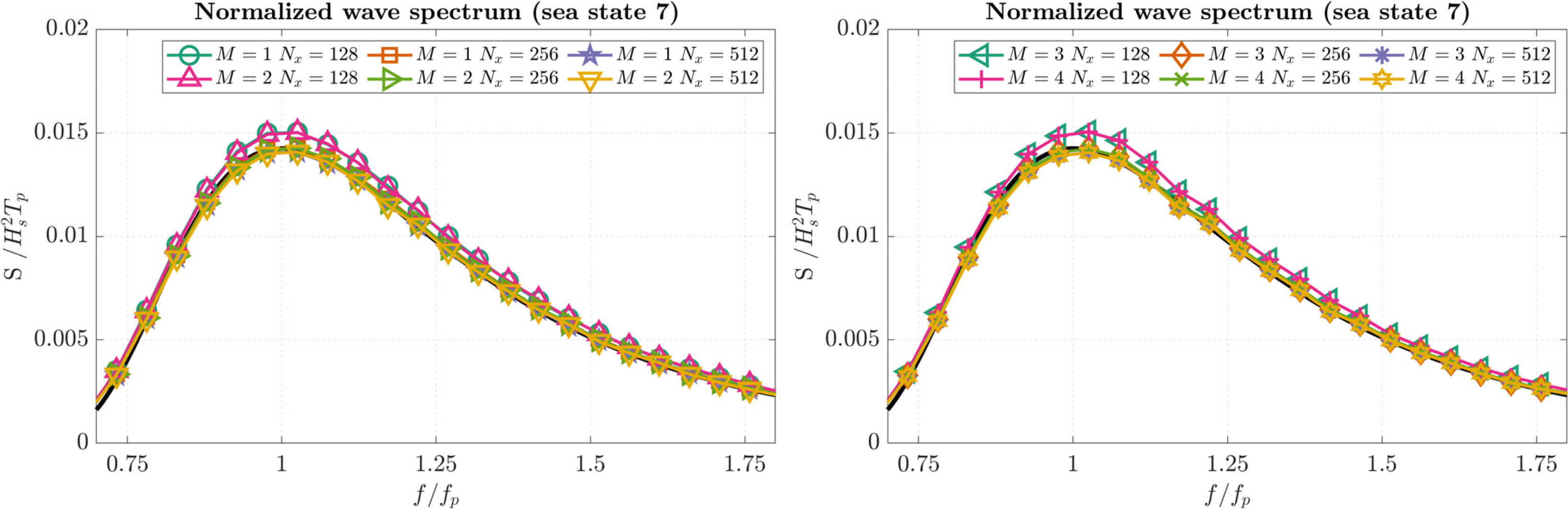
Normalized wave spectra of sea state 7 with different combinations of HOS parameters
The difference ratio of each wave spectrum is compared. Fig. 4 illustrates the difference ratio of the wave spectrum with respect to the angular frequency. The tolerance criterion of the wave spectral analysis is ±5% within the frequency range f ∈[0.75fp; 1.5fp ], where fp is the peak frequency of the target sea state. Note that this spectral qualification criterion was adopted from previous studies (Canard et al., 2020; Canard et al., 2022). The red-colored region presents the target tolerance zone. First, the wave spectra obtained with Nx = 128 were overestimated compared with the target spectra for all sea states regardless of the HOS order. For all combinations of the HOS parameters except for the HOS modes Nx = 128, the difference ratio of wave spectrum lie in the ±5% tolerance within the target frequency range. A comparison of the difference ratio with respect to the HOS order revealed a relatively large variation as the HOS order increases.
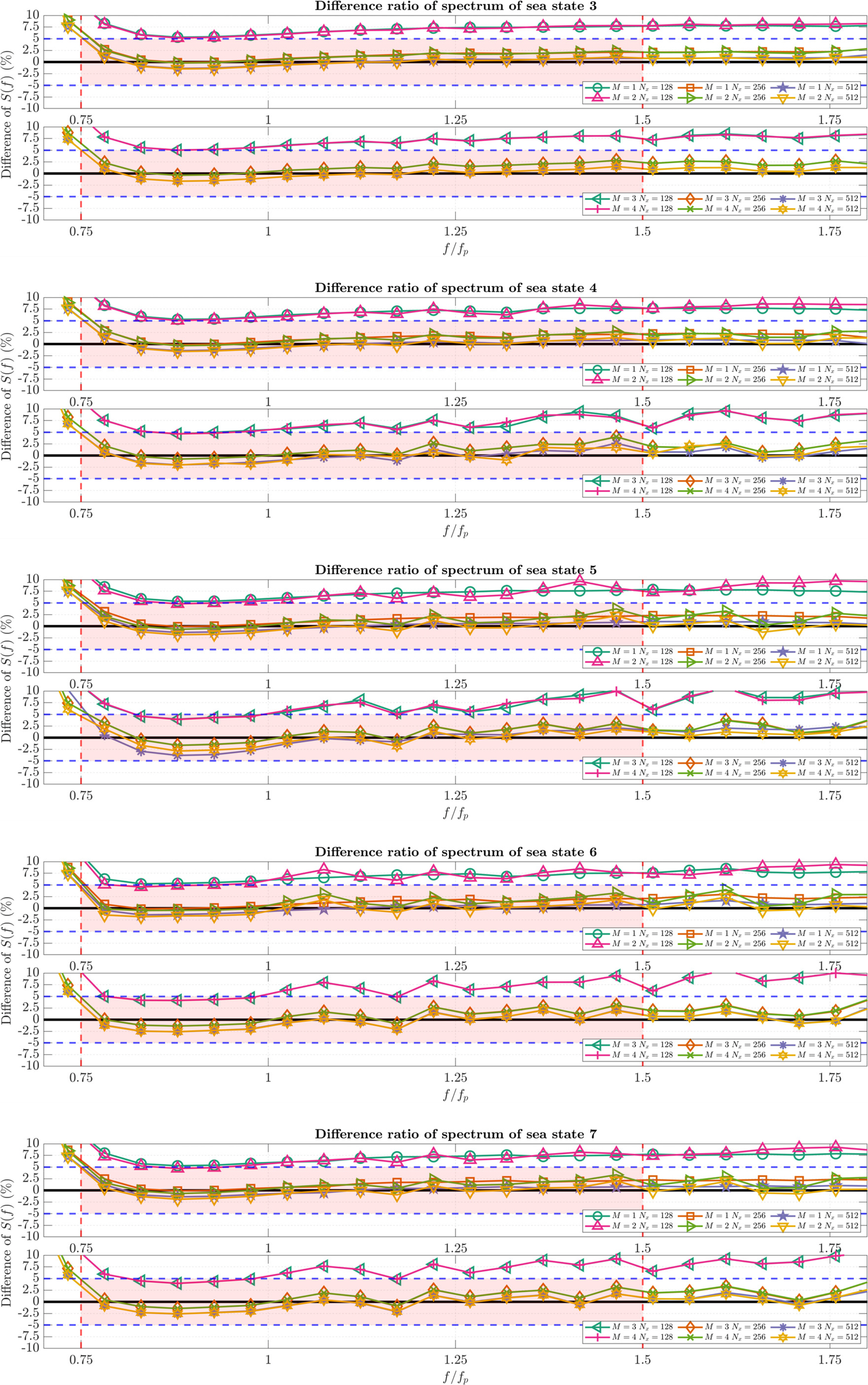
Difference ratio between the measured wave spectrum and the target wave spectrum. The red zone is the target tolerance zone.
A quantitative comparison of the wave spectrum for each HOS computational parameter was conducted. The maximum difference ratio and the average absolute difference ratio of the wave spectrum in the target frequency range were evaluated using Eqs. (15) and (16), and the values are presented in Table 3.
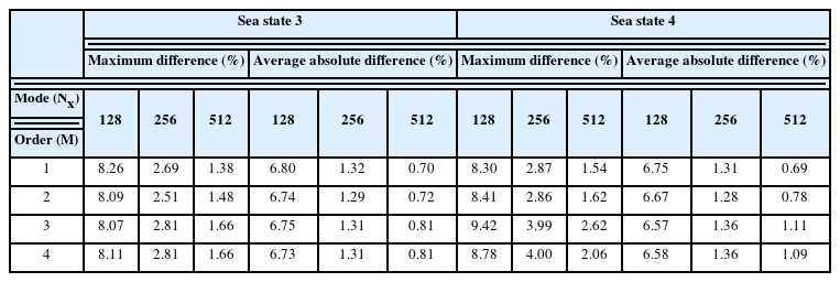
Maximum and averaged difference of wave spectrum with respect to sea states and HOS parameters
Table 3 lists the computational setup where their maximum and averaged absolute difference ratio is larger than 10% is colored red, larger than 5% is colored yellow, and less than 5% is colored green. As shown in Fig. 4, all results with HOS modes Nx = 128 have maximum and average absolute difference ratios larger than 5%. The difference ratio decreased as the number of modes increased. In addition, the difference ratio tends to increase as the HOS order increases, but the increment is relatively small.
For all sea states, the smallest average absolute difference ratio was measured with the computational setup of HOS modes Nx = 512 and HOS orders M = 1. The largest maximum difference ratio with HOS modes Nx = 256 was 4.00% (sea state 4, Nx = 256, M = 4), and the largest maximum difference ratio with HOS modes Nx = 512was 3.82% (sea state 5, Nx = 512, M = 3). The largest average absolute difference ratio with HOS modes Nx = 256 was 1.58% (sea state 5, Nx = 256, M = 3), and the largest average absolute difference ratio with HOS modes Nx = 512 was 1.58% (sea state 5, Nx = 512, M = 3). The average absolute difference ratio with HOS modes Nx = 256 and Nx = 512 was suppressed by under 2%. In addition, approximately 1% of the average absolute difference ratio is measured with HOS mode Nx = 512 and HOS order M = 2. Therefore from the spectral analysis, the HOS modes Nx = 512 is recommended for the HOS wave generation.
4.2 Wave Crest Probability Distribution Analysis
As discussed in the Introduction, both the PDSR and the PDER of the HOS waves were compared with the Rayleigh (first-order), the Forristall (second-order), and the Huang (semi-empirical formula) distributions. Eqs. (17)–(19) describe the mathematical formula of the Rayleigh, the Forristall, and the Huang distributions, respectively. Each distribution describes the POE of the measured wave crest from the mean free surface (ηc). In Eq. (20)Ur is the Ursell number, S1 is the steepness parameter, k1 is the wavenumber, T1 is the mean wave period, and d is the water depth. The Huang PDSR and PDER coefficients in Eq. (19) are summarized in Table 4.
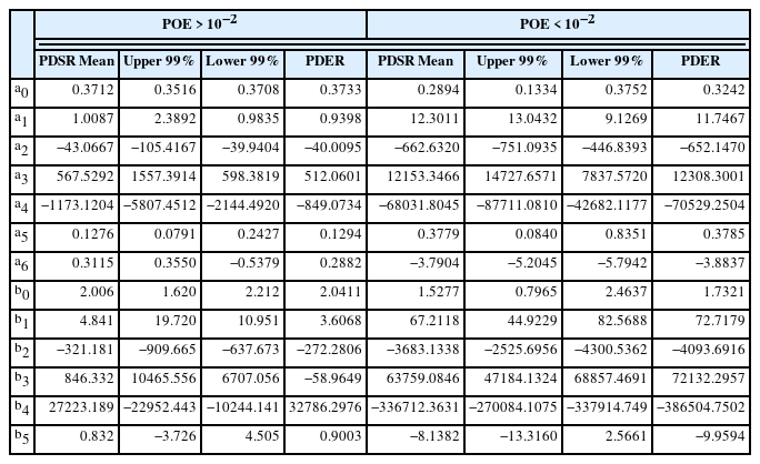
Coefficients for Huang semi-empirical PDSR and PDER formula
Fig. 5 presents the PDSR curves from 100 realizations and compares them with the reference distributions. Each graph presents a sea state, and every subplot presents a combination of HOS parameters. The name of each computational setup is written inside the subplot, and all subplot shares the same axis limits. Each marker presents a wave crest height probability, and the mean PDSR curve is an average of all wave crest height probability distributions from 100 wave realizations. The analyses of the PDSR markers and the mean PDSR curve are described as follows
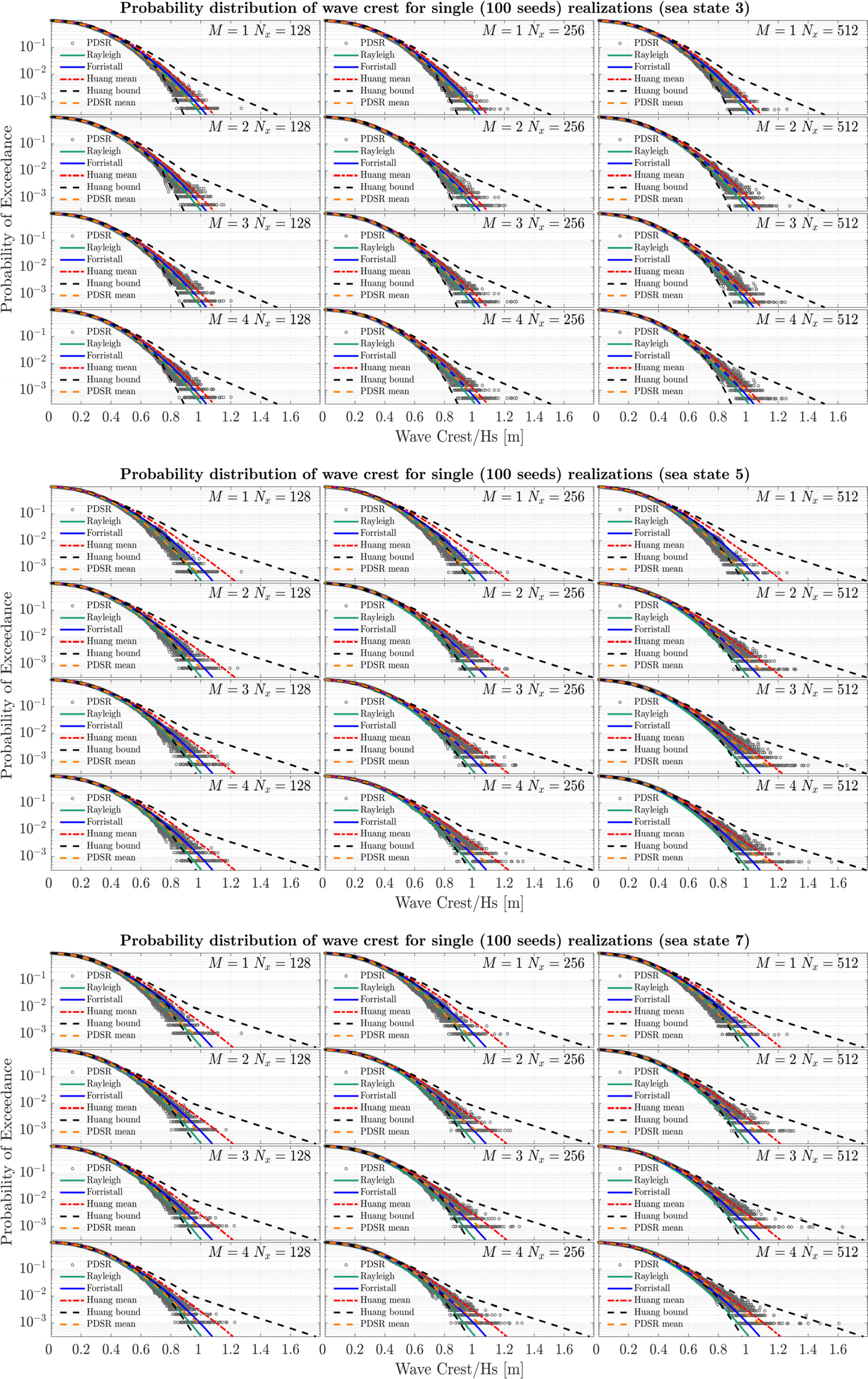
PDSR and mean PDSR of 100 realizations made with different combinations of HOS parameters for sea states 3, 5, and 7. These were compared with the Rayleigh (first-order), the Forristall (second-order), and the Huang (semi-empirical formula) distributions.
First, the PDSR markers and the mean PDSR curves were compared with the reference distributions. With the HOS mode Nx = 128, the change of HOS order did not influence the mean PDSR curves significantly, and the mean PDSR curves mostly follow the Rayleigh distribution regardless of the wave condition. With HOS modes Nx = 256 and Nx = 512, a meaningful difference was measured with the change in the HOS order. When the first-order (M = 1) was applied, the mean PDSR curves followed the Rayleigh distribution regardless of the number of HOS modes. When the second-order (M = 2) was used, the mean PDSR curves followed the Forristall distribution. This trend was presented more distinctly for the higher sea states.
The third-order (M = 3) and the fourth-order (M = 4) HOS simulations with HOS modes Nx = 256 and Nx = 512 were compared for sea states 5 and 7. The mean PDSR curves mostly lied between the Forristall distribution and the Huang mean distribution. The mean PDSR curve showed a significant increase as the number of HOS mode increased. Moreover, the variations of the PDSR markers from the mean PDSR curve has changed as the number of HOS mode increased. For example, in the case ‘sea state 7/M = 4/Nx = 256’ and ‘sea state 7/M = 4/Nx = 512’, the number of PDSR markers under the Huang 99% lower bound decreased, and the number of PDSR markers close to the Huang 99% upper bound increased. This result suggests that HOS mode Nx = 512 is required to generate extreme wave events. One reason for this variation of PDSR markers is the increase in the Nyquist frequency and the increase in HOS mode. The increase in Nyquist frequency leads to more proper modeling of high-frequency wave components and the nonlinearity of waves.
Second, the PDSR markers were compared with the Huang 99% bounds. Considering the concept of the Huang 99% bounds, the PDSR markers are expected to mostly be in the Huang 99% bounds. Therefore, the analysis counts all wave crest heights with their POE lower than 10−2 and compares them with the Huang bounds. Table 5 lists the occurrence rate of the measured wave crest height POE not being inside the Huang bounds for POE lower than 10−2 for each sea state and each HOS computational parameter. The computational setup with an occurrence rate higher than 10% is colored red, higher than 5% is colored yellow, and lower than 5% is colored green (Table 5).

Occurrence rate of the measured wave crest height POE not being inside of the Huang bounds for POE lower than 10−2.
For sea states 3 and 4, which are almost linear wave conditions, the influence of HOS parameters was smaller than in the other sea states. On the other hand, for the sea states 5 to 7, more than half of the PDSR markers measured from first-order (M = 1) HOS simulations were lower than the Huang 99% lower bound. The occurrence rate gradually decreases as the HOS order increases from M = 1 to M = 3. While the difference between M = 3 and M = 4 was minimal. Similarly, the occurrence rate decreases as the number of HOS modes increases. The lowest occurrence rate for each sea state was commonly found with HOS setup M = 3/Nx = 512 or M = 4/Nx = 512, and those values were retained under 2%.
Fig. 6 compares PDER curves of 100 realizations and the reference distributions for sea states 3, 5, and 7. An additional reference distribution presenting the 5% bound of the Huang ensemble distribution was added as an indicator. For sea states 3, due to the lack of nonlinearity, the difference between each PDER curve with different computational setups was smaller than the other sea states. For sea states 5 and 7, a significant change in wave crest height was observed, particularly at the POE level of 10−5.

PDER of 100 realizations with different combinations of HOS parameters for all sea states. These are compared with the Rayleigh (first-order), the Forristall (second-order) and the Huang (semi-empirical formula) distributions.
The PDER curves obtained from the first-order HOS simulations for all sea states agree well with the Rayleigh distribution. The PDER curves of the second-order HOS simulations matched well with the Forristall distribution when the number of HOS modes was higher than Nx = 256. The third- and fourth-order PDER results usually lie between the Forristall distribution and the Huang PDER distribution, while the difference between the two HOS orders is minimal. The M = 3/Nx = 512 and M = 4/Nx = 512 setups showed the best compromise among all HOS computational setups with the Huang ensemble distribution. Within the POE level between 10−2 and 10−4, the HOS PDER curves follow the −5% bound of Huang ensemble distribution. Within the POE level between 10−4 and 10−6, HOS PDER curves show overestimated wave crest probability compared to the Huang ensemble distribution. On the other hand, the number of realizations is insufficient to conclude the PDER curve’s accuracy at the POE level of 10−5.
5. Conclusions
This paper performed a parametric study on the open-source program HOS-Ocean. With three numbers of HOS modes (Nx ) and four levels of HOS orders (M ), twelve combinations of HOS computational parameters were applied to the HOS simulations to find the recommended HOS parameters for irregular wave generation. Therefore, 100 three-hour realizations of HOS waves were made for five sea states, and the quality waves were verified by following qualification procedures.
First, the spectral analysis was performed with twelve combinations of HOS setup and five sea states, and the averaged wave spectrum was compared with the target wave spectrum. The maximum and average spectral differences were quantitatively analyzed within the target frequency range using ±5% tolerance. Second, the nonlinearity of irregular waves with respect to the HOS parameters and the variation of sea states were checked by comparing the POE of the wave crest height. The PDSR and PDER of 100 realizations were compared with the reference probability distributions, and the influence of HOS parameters and sea states on the nonlinearity of irregular waves was investigated. As a result, the following conclusions were acquired.
The results with HOS modes Nx = 128 show overestimated wave spectrum and underestimated wave crest height regardless of the HOS order. Consequently, the HOS mode was larger than Nx = 128 is required for the current HOS computational setup, regardless of the sea state.
The minimum spectral difference (averaged absolute difference ratio) was found when the first order was applied. The spectral difference increases as the HOS order increases. On the other hand, regardless of the HOS order and the sea state, the maximum difference ratio was maintained below 5%, and the averaged absolute difference ratio was kept below 2% with HOS modes Nx = 256 and Nx = 512.
The wave crest height PDSR and PDER for different combinations of HOS parameters were compared with the reference distributions.
When the first-order HOS order was used, the wave crest height was significantly underestimated even for sea states 3 and 4. This underestimation clearly showed that it is important to check both the wave spectrum and the wave crest height POE for the irregular wave analysis.
Comparing the PDSR of the second-, third-, and fourth-order HOS simulation with the Hunag 99% bounds, the HOS wave crest generated using two combinations of HOS parameters M = 3/Nx = 512 and M = 4/Nx = 512were considered adequate for all sea states. For sea state 3, other HOS setups, such as M = 2/Nx = 256 or M = 2/Nx = 512 were considered appropriate.
The HOS setups, M = 3/Nx = 512 and M = 4/Nx = 512, satisfy the ±5% tolerance in the spectral analysis. The amount of nonlinearity of waves measured using the two HOS setups was verified by comparing the wave crest height POE with the Huang PDSR and PDER distributions. The difference in wave properties between the two HOS setups was small. In conclusion, considering that the HOS domain length is 15λp, the suggested HOS computational parameter would be λp/Δx ≧ 35 with M = 3.
Notes
No potential conflict of interest relevant to this article was reported.
This work was supported by Pusan National University Research Grant, 2021 and supported by BK21 FOUR Graduate Program for Green-Smart Naval Architecture and Ocean Engineering of Pusan National University.