Underwater Navigation of AUVs Using Uncorrelated Measurement Error Model of USBL
Article information

Abstract
This article presents a modeling method for the uncorrelated measurement error of the ultra-short baseline (USBL) acoustic positioning system for aiding navigation of underwater vehicles. The Mahalanobis distance (MD) and principal component analysis are applied to decorrelate the errors of USBL measurements, which are correlated in the x- and y-directions and vary according to the relative direction and distance between a reference station and the underwater vehicles. The proposed method can decouple the radial-direction error and angular direction error from each USBL measurement, where the former and latter are independent and dependent, respectively, of the distance between the reference station and the vehicle. With the decorrelation of the USBL errors along the trajectory of the vehicles in every time step, the proposed method can reduce the threshold of the outlier decision level. To demonstrate the effectiveness of the proposed method, simulation studies were performed with motion data obtained from a field experiment involving an autonomous underwater vehicle and USBL signals generated numerically by matching the specifications of a specific USBL with the data of a global positioning system. The simulations indicated that the navigation system is more robust in rejecting outliers of the USBL measurements than conventional ones. In addition, it was shown that the erroneous estimation of the navigation system after a long USBL blackout can converge to the true states using the MD of the USBL measurements. The navigation systems using the uncorrelated error model of the USBL, therefore, can effectively eliminate USBL outliers without loss of uncontaminated signals.
1. Introduction
The ultra-short baseline (USBL) acoustic positioning system measures the bearing angle and slant angle of the received acoustic signal and converts the propagation delay time of the sound wave into a distance. It is an underwater acoustic positioning device that measures the relative position of an underwater object via a triangulation method using two angles orthogonal to the distance (Milne, 1983). The USBL system has advantage of being convenient for operation owing to its ability to measure the position of an underwater object using a single transceiver. For this reason, it is widely used for the location tracking of remotely operated vehicles and autonomous underwater vehicles (AUVs). In addition, the USBL can measure the position of the underwater object within a certain error bound regardless of the elapsed time. It is also employed as an auxiliary sensor for aiding the navigation systems of underwater vehicles composed of inertial sensors (Vasilijevic et al., 2012; Lee et al., 2017).
To use the USBL position measurements for aiding a navigation system, an error modeling system of the USBL is required. The main sources of errors are the physical properties of the acoustic propagation medium, diffraction, and non-uniform underwater environments (temperature gradient, pressure gradient, etc.). So characteristics of the errors varies depending on factors such as multi-pass of acoustic propagation, variation of ambient noise caused by passing ships, unique features of the transceiver array (i.e. range-dependent error in the angular direction), and misalignment of the transceiver mounted on the vehicle frame. The USBL is particularly sensitive to noise because it measures the reception angle to calculate the phase difference of the signal received by the transceiver array (Luo et al., 2021). This makes the USBL prone to outliers. Since the USBL’s position error increases in proportion to range, the position measurement in the horizontal plane shows nonlinear tendencies when the operating depth is smaller than the measurement range. The USBL, in case of which tracks the positions of underwater vehicles operated in shallow water, has an elliptical distribution of measurement errors according to the distances from the reference station to the AUVs. Furthermore the principal axis of the elliptical distribution changes according to the positions of the vehicles relative to the reference station. Therefore, when USBL positioning measurements are used for aiding an underwater navigation system of an underwater vehicle operating in shallow water, a measurement model including the nonlinear characteristics of the errors is required. In particular, it is essential to design a filter that can selectively reject outliers for a robust navigation system. To utilize the USBL signal for the navigation system even in abnormal situations, such as blackout or frequent outliers of USBL measurements, it is necessary to ensure the stability of the navigation system with outlier rejection and reduce the position errors after when the USBL signal reception is recovered from the blackout. For example, as shown in Fig. 1, USBL tracking of the locations of AUVs operating under an ice shelf requires not only the rejection of outliers but also decision on integrity of the USBL signals received after a long time of blackout (Park, 2021).
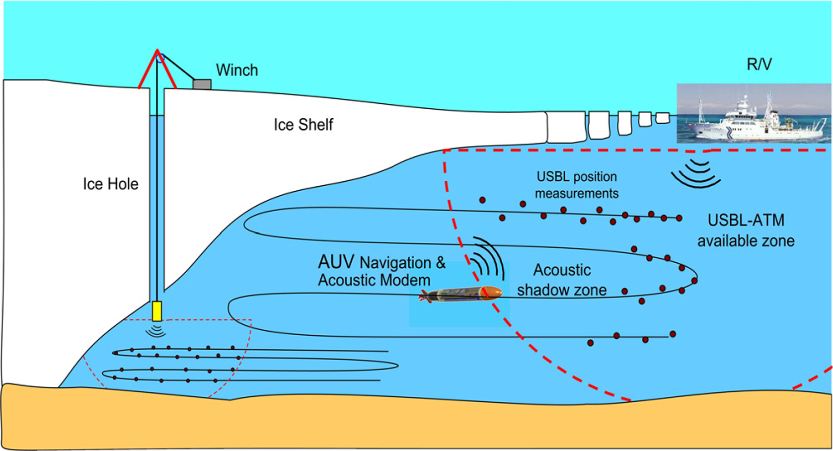
Integrated navigation aided with a USBL and an acoustic telemetry modem for exploration of the Antarctic Ocean under an ice shelf
An AUV position measured by USBL is defined using the Earth coordinates. However, the acceleration, angular velocity, and speed used in the navigation of the AUV are defined using the body-fixed coordinates of the vehicle. The position measurement tolerance of the USBL can be modeled in the Earth coordinate system by separating the direction toward the vehicle and the direction orthogonal thereto. As the vehicle moves, the position and heading change constantly. So, the three-dimensional (3D) error component of the USBL defined in the body coordinate system of the vehicle changes according to the attitude and heading of the vehicle. To use the USBL position signal as an auxiliary signal for aiding a navigation of the vehicle, it is necessary to transform the global coordinate to the body frame of the USBL measurements. The error covariance of the USBL defined in the body coordinate system of the vehicle is correlated between the coordinate axes. When this correlation error covariance model is applied to the navigation system, the outlier decision level should be set to large values, ensuring that the normal USBL signals are not lost. If the navigation system is designed in such a way, outliers within the threshold, which have to be rejected, can be recognized as signals. Therefore, the outlier determination area should be minimized so that only the outliers are rejected while normal signals are secured. Uncorrelated error modeling is one of the potential methods for reducing the outlier decision area.
In the studies on outlier rejection, De Maesschalck et al. (2000) defined the Mahalanobis distance (MD) and determined its relationship with the Euclidean distance (ED) through principal component analysis (PCA). They explained and discussed the techniques based on the MD and outlier rejection applied in multivariate calibration, pattern recognition and process control. Chang (2014) proposed a robust Kalman filter to reject the outliers from the measurement signal. By assuming that the difference between the measured signals containing noise and the estimated state was a Gaussian distribution, he set outlier judgment indices and statistically treated them as null hypotheses to perform tests on actual observations. In the case of outliers, a scale factor was introduced to readjust the covariance of measurement noise, and a solution was obtained using Newton's repetitive method or an analytical method. However, this approach may not be practical if the number of repetitions increases. Hassan et al. (2021) proposed a method for rejecting outliers via repeated smoothing process with an image signal and a low-cost inertial sensor in underwater. By installing reference markers on an underwater structure and updating the innovation and covariance when the acquired image information is valid, they showed that outliers can be removed and navigation accuracy can be improved through experiments. Zhu et al. (2021) proposed an improved Kalman filter algorithm based on MD algorithm to deal with outliers. For a strap-down inertial navigation system (SDINS) aided with a DVL, the adaptive and robust estimation of the error covariance was developed to suppress the effect of the non-Gaussian noise. To design the robust filter adapting to the environment, they used an MD algorithm for the DVL signal containing the non-Gaussian noise. A simulation was performed using the in-flight alignment test data of the DVL-aided SDINS. They showed that the covariance matrix could be adaptively estimated in real time and the outliers could be effectively suppressed.
This paper proposes a method of modeling the measurement error of USBL as an uncorrelated error in the horizontal plane for the design of a robust underwater vehicle navigation system to outlier, which uses MD and principal component analysis of the USBL error model. Using this method, the error characteristics of the USBL positioning data can be decomposed and set to the principal axis of normal distribution in the MD. We analyzed the feature of position measurements of the USBL and modeled the inherent error characteristics of the USBL measurement system accordingly. The difference between the position estimated by the navigation system of the vehicle and the measured position was updated with a Kalman filter having the modulated error covariance of measurements on the basis of the MD. To evaluate performance of the outlier rejection with the error model, a simulation on the underwater navigation of an AUV was conducted with a data set of surface maneuvering test of the vehicle. This paper investigated the robustness of the outliers rejection among the USBL measurements as well as the effects of the varying magnitude and direction of the measurement error covariance on the performance of the navigation system . Through the simulation of the navigation aided by USBL measurements, it was confirmed that the proposed method is more robust to reject outliers than a conventional method. This paper also examined that the erroneous estimation of the navigation system after a long USBL blackout can converge to the true states using the MD of the USBL measurements.
2. Underwater Navigation Aided with USBL
2.1 Position Measurements of USBL in the Horizontal Plane
USBL is performed by measuring the bearing angle ψbearing and the slant angle θslant of the two directions that are orthogonal to each other as well as the time delay of the transmitted-received signal δT, as shown in Fig. 2. If the sound velocity c is known, the relative three-dimensional position in underwater can be calculated with one range R (= cδT/2) and two angles ψbearing and θslant. When the water depth is greater than the horizontal distance, the horizontal position measurement error can be assumed to have independent normal distributions in the x- and y-directions. In this condition, the USBL system has been successfully applied to aiding a navigation system as an auxiliary sensor in a previous study (Lee et al., 2017). If an AUV is performing a long-range exploration in an ice sheet or operating in a shallow water, the error in the radial direction will be constant regardless of the range as well. However, the error in the angular direction that is perpendicular to the radial direction will increase with range. Therefore, an error modeling approach of the USBL able to handle this feature should be developed for aiding underwater navigation in shallow water.
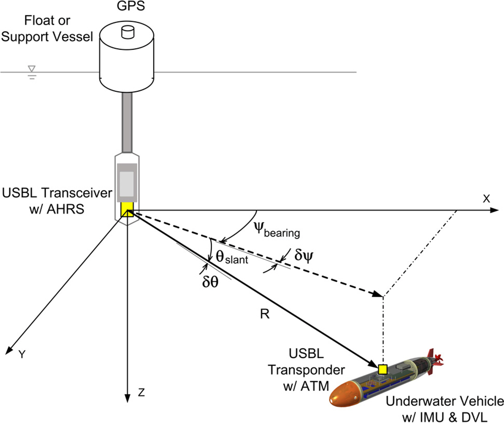
Angular measurement errors of the USBL acoustic positioning system
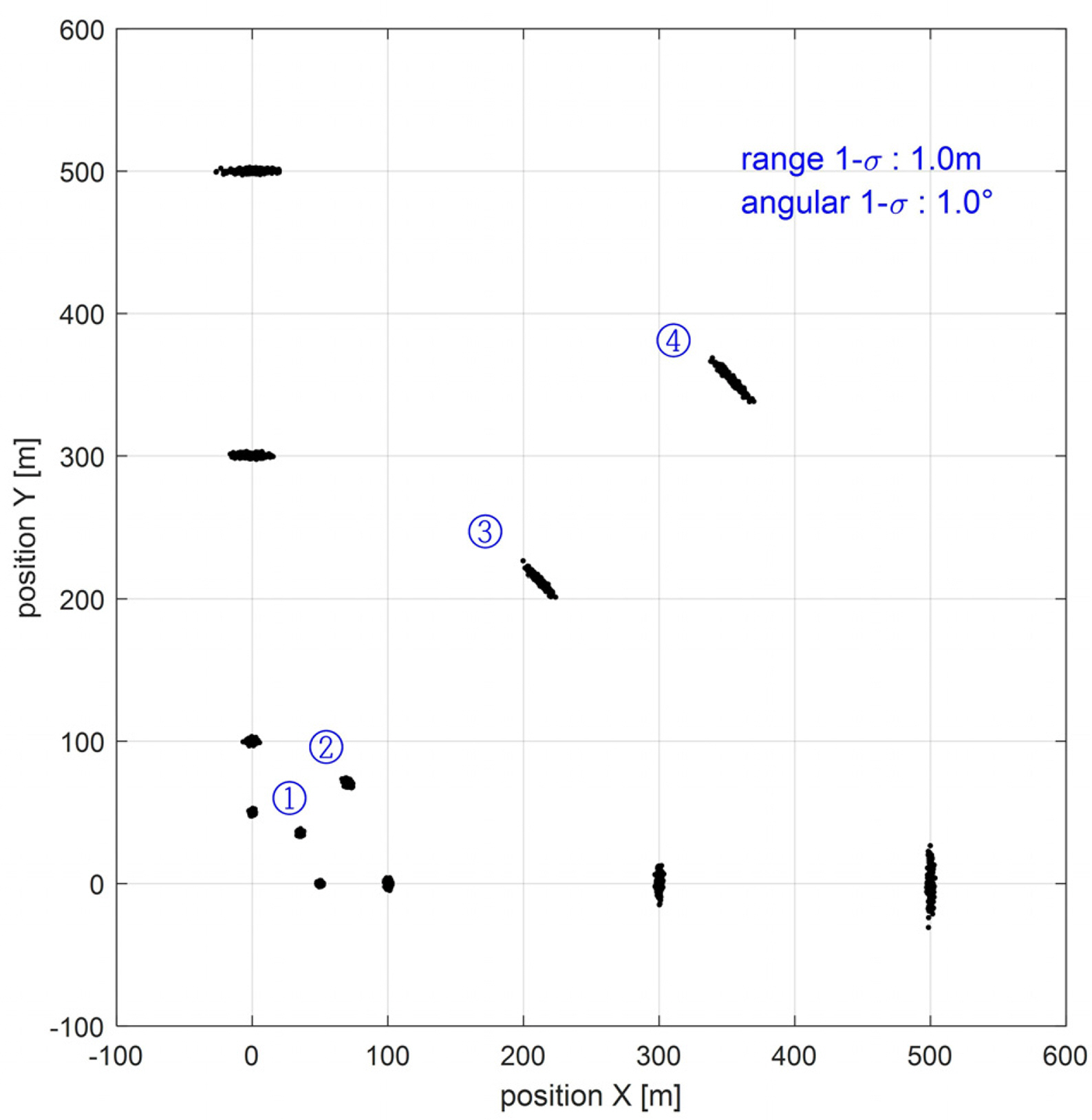
In this article, the MD is introduced for the error modeling of measurement equations of USBL. Considering the characteristics of commercially available USBL 18/34 (EvoLogics, 2017), a virtual USBL measurement data set was generated whereby the characteristics of each location were analyzed. A simulation was performed for the cases where the rms error of range was 1 m and the rms error of angle was 1°, in which it was assumed that the range error and angular error of the USBL had a normal Gaussian distribution. In such cases where an underwater vehicle operating at a depth of 10 m was stationary at a horizontal distance of 50, 100, 300, or 500 m from a reference station with 0°, 45°, and 90° bearing angles centered on the USBL transceiver on the station, a series of data set was simulated to track the stationary vehicle at each location with the USBL. These data were generated with random noise following a normal distribution, assuming a 10-min measurement at 2 samples per second. The number of each dataset is 300. Fig. 3 shows the simulated positions of the USBL measurement for 12 locations. As the relative range increased, the error in the direction perpendicular to the radial direction increased linearly, and the principal axis of the elliptical error distribution changed according to the relative bearing angle. The left column of Fig. 4 presents an enlarged view of the position measurement data at each position for points ①–④ with a 45° bearing angle. Here, the angular direction error of the simulated positions of the USBL exhibits a distorted oval-shaped distribution and increases in proportion to the range of the vehicle. In the figure, the concentric ellipses represent the contours equivalent to (σ1, 2σ1, 3σ1 ) of the standard deviation σ1 of the first principal component (PC1) for each position dataset. Because the error distribution of the USBL measurement has nonlinear characteristics, underwater vehicles operating in shallow water require an error modeling to consider the correlation between the x- and y-axis directions.
Simulated USBL measurements with root-mean-square (rms) errors of the heading and range (δψ = 1°, δr = 1 m) at a depth of d = 10 m
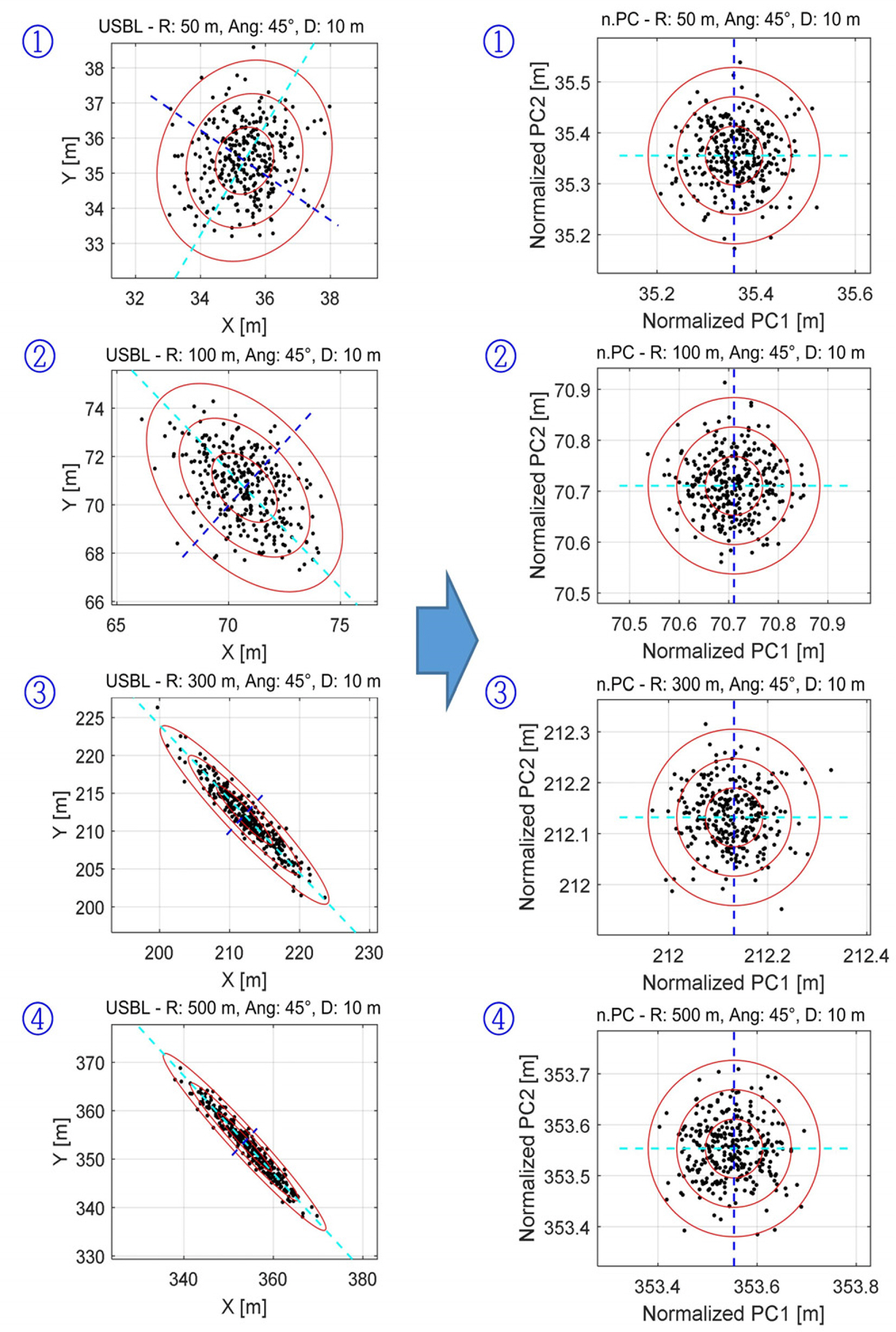
(Left) measurement errors at positions ① to ④ in Euclidean space, (right) normalized principal components (PCs) of the measurements in the Mahalanobis distance
2.2 MD and PCA of the USBL Measurements
The MD and PCA were reviewed prior to modeling the USBL position data. Assuming that the USBL localization error has a normal Gaussian distribution with mean μ and covariance Σ, the probability density function of the k-dimensional multivariate vector X = (X1,…,Xk)T is expressed as follows:
Here, σ1 and σ2 represent the standard deviations of the principal components, and ρ12 represents the correlation coefficient between x1 and x2 . If the standard deviations in the x- and y-axis directions are equal, the MD is equal to the ED (MDi = EDi ).
For the PCA, consider a data matrix of X (n×p) that includes n measurements (xi ) composed of p variables. Xc is determined by removing the mean x̄j from each column vector xj(n×1) in the data matrix X (n×p). In this sense, if singular value decomposition is performed, Xc can be expressed as
When applied to the position measurement data of the USBL, the position data on the horizontal plane are 2-D; thus, p = 2, a = 2, and the USBL dataset, i.e., (x, y), can be handled using the PCA. The average of the position dataset is calculated and eliminated, and the PCA can be performed on the matrix Xc as follows, by using the singular value decomposition of the MATLAB function svd().
Here, S represents the diagonal matrix of the singular values Λ . The right column of Fig. 4 indicates that the normalized MD data of the USBL position error of points ①–④ have a 2-D symmetric normal distribution. As shown in Table 1, as the range increases, the first singular value of the PC (PC1) increases proportionally (0.99, 1.75, 5.55, and 8.55). However, the singular value of the second PC (PC2) does not change significantly. In Fig. 4, concentric circles represent the equidistance of the Mahalanobis distance MD, 2MD, and 3MD corresponding to σ1, σ2, and σ3, respectively.

Standard deviation for the principal axis of the relative position of the USBL
2.3 USBL-aided Navigation System of AUVs in Shallow Water
The objective of this study is to design a navigation system robust to outliers using the USBL position information for the operation of AUVs in shallow waters. Since the error characteristics of the USBL change according to the relative range and direction between the transceiver of the USBL and the AUVs, it is necessary to make an uncorrelated error model of the USBL to provide auxiliary measurement information in the navigation system. The navigation system of the vehicles equipped with inertial sensors can be modeled in various forms depending on the grade of the sensors. In this study, a dead-reckoning navigation method was applied to estimate the position. The simple equation of motion was established using only the speed, bearing angle, and position information of the AUV (Lee et al., 2017). If the AUV operates at a constant speed and the accelerations of the vehicle can be assumed decoupled normal noises in each direction, the equation of motion can be expressed as follows:
Here, yk is the measured states, the measurement matrix Hk = [I7×7 07×1]. We assumed that the noise vector is the normal distribution vk ∼ N (0, Rk ) where the mean is zero and the covariance matrix Rk is
If we assume that the horizontal position Xk and Yk is not correlated with other state variables, we can separately handle the covariance matrix Rxyk of the x and y position derived from the error of the USBL measurements. Then the covariance matrix can be expressed as follows in the horizontal plane:
An arbitrary vector x can be converted into an arbitrary coordinate x̃ using the unitary matrix Φ (ΦH Φ =I). If x̃ is defined on the principal axis of the ellipse representing the error covariance of the USBL position measurement, it can be expressed as x = ϕ1 x̃1 + ϕ2 x̃2 in the horizontal 2-D plane. Fig. 5 illustrates an example of matching the eigenvector to the main axis of the error covariance of the USBL measurements. In the figure, ϕ1 and ϕ2 are the eigenvectors of the error covariance matrix matched to the principal-axis of the error distribution.
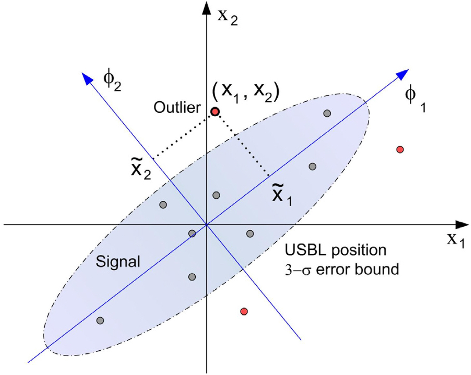
Rotation of the axis using a unitary matrix
Because the error covariance of the USBL measurement Rxyk is a Hermitian matrix, the eigenvalues can be decomposed into a diagonal matrix of Rxyk = Φ Λ ΦH (Scharlau, 1985), where
Therefore, the error covariance, which is correlated depending on the relative position and angle of the vehicle with respect to the USBL reference station, is decorrelated by transforming its axis to the principal component axis. And then the decorrelated error covariance can be used for implementing the USBL-aided navigation. If the error of the USBL measurement is located outside a certain bound, e.g., 3-σ illustrated in Fig. 5, we can decide that the USBL measurement is an outlier.
The integrated navigation system aided with the USBL was developed using the Kalman filter (Gelb, 1974; Simon, 2006). Fig. 6 shows a configuration diagram of the navigation system implemented in this study. The simulations of the navigation system were performed by updating the system error covariance with the innovation which is the difference of the estimated position and the USBL measurement with outlier. Assuming that the effect of time delay of the position data transmitted through an acoustic telemetry modem was compensated by the dead-reckoning navigation in a short interval, the time delay was not considered in the simulations.
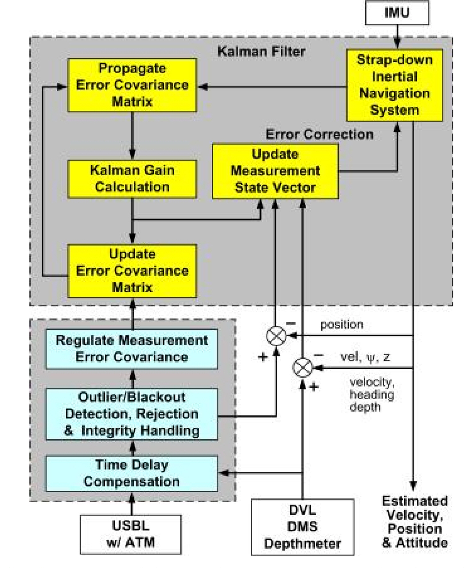
USBL-aided integrated navigation system based on the inertial measurement unit and DVL with the uncorrelated USBL error model and outlier rejection
3. Underwater Navigation with the Uncorrelated Error Model of USBL
3.1 Motion Data of an AUV and Simulation of the USBL Measurements
A navigation simulation involving the USBL outlier rejection algorithm was performed using a dataset of the 1-hours surface navigation of an AUV owned by Hanwha Systems Co., Ltd. The experiment was conducted at surface by reciprocating an arbitrary short-range path within Jangmok Bay at Jeoje Island. The sensors equipped on the AUV were a global positioning system (GPS), an inertial measurement unit (IMU FI200P), a Doppler velocity log (DVL RDI), an attitude heading reference system (AHRS) (TCM-XB), and a depth meter. To realize a situation in which a large navigation error occurred during blackout, a dead-reckoning navigation system integrated with the horizontal velocities and heading angle was introduced. The uncorrelated error model of USBL was applied to the navigation system. Fig. 7 presents the experimental data of the AUV used in the simulation. Fig. 7(a) shows the forward, lateral and vertical velocities measured by the DVL, u, v, w ; Fig. 7(b) shows the AUV’s latitude and longitude measured by the GPS, y and x, and Fig. 7(c) shows the heading, roll and pitch angles of the AUV by the AHRS. All the sensor information was stored at 100 sps (samples per second) rate, and the sampling rate of the DVL was 10 sps.

Experimental data used in the simulation for the integrated navigation: (a) Velocity of the vehicle in the x, y, and z direction; (b) Y and X positions; (c) Attitude of the vehicle
The experiment was performed on the sea surface to acquire the absolute position with the GPS, so the USBL measurement was not conducted. Instead, the USBL positioning data was simulated by adding the errors, generated with the stochastic features of the USBL sensor and a certain bound of outlier, to the absolute position. We used the specifications of the USBL EvoLogics 18/34 in the simulation and produced the USBL positioning data from a reference station to the current position of the vehicle at every 2 seconds. Additionally, we supposed the outlier ratio of the USBL would be set as 20%, so the outlier was generated at 10-seconds interval. The bearing-angle error of the USBL was set as 1.0° rms to consider the heading sensor specifications of the USBL built-in AHRS, as shown in Table 2. The range error of the USBL was set as 1.0 m rms to consider the motion compensation error of the moving vehicle and the variation of the acoustic propagation media. The outliers were generated by adding uniformly distributed random variables in [0, 30] m displacement and in [0, 360]° angle, which is independent of the current position of the vehicle.
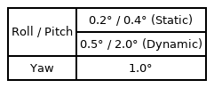
Specifications of the AHRS of the EvoLogics USBL
Fig. 8 shows the USBL positioning data generated according to the AUV trajectory as Fig. 7(b) in case of no outlier, where the initial position of the vehicle was set at (0, 0) and the reference station of the USBL transceiver was located at (−100, 300). The error increased in the direction perpendicular to the radial direction as the distance from the reference station to the USBL increased. The error of the simulated USBL measurements increased in the orthogonal direction of the radial axis of the range from the reference station to the vehicle as the range increased. In addition to changing the magnitude, the principal axis of the error changed according to the location of the reference station. Fig. 9 shows the process of generating the simulated error of the USBL measurements: The upper parts are the simulated position error of the USBL measurements in the x- and y-directions; The middle parts are outliers generated as explained previously; The lower parts show the simulated error of the USBL measurements including the two components of the errors.

USBL measurements generated by adding normal angular and range errors to the GPS positions
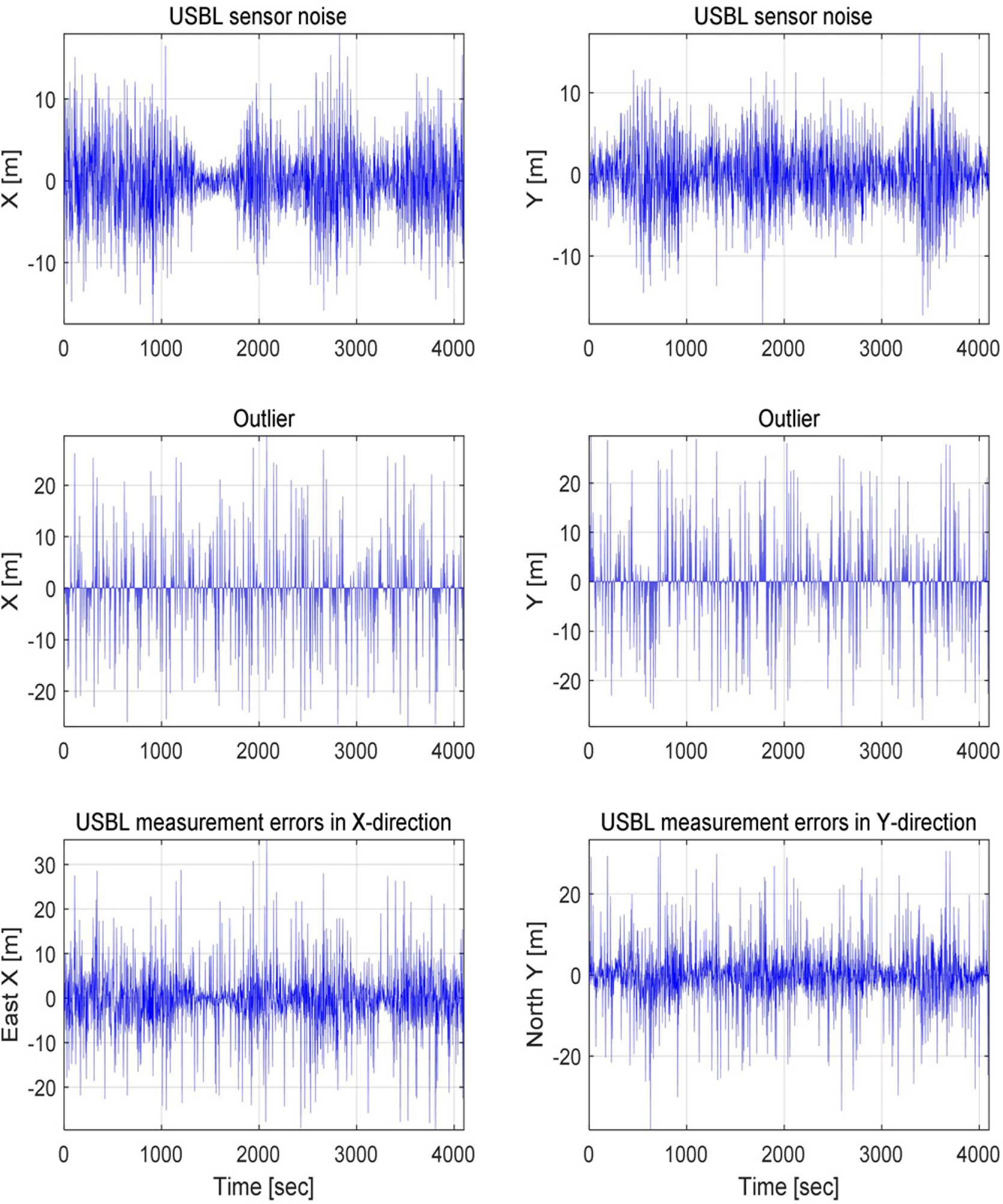
Simulated USBL measurements with outliers: (top) intrinsic errors of the USBL—0.5 sps with Gaussian noise in the range direction and the orthogonal direction thereto; (middle) outliers—0.1 sps with uniform noise in the distance range of [0 30] m and the angular range [0, 360]°; (bottom) simulated errors. USBL measurements were generated by adding GPS measurements to these errors.
3.2 Simulation of USBL-aided Underwater Navigation with the Uncorrelated Error Model
A simulation was performed for the USBL-aided navigation system with the uncorrelated error model of USBL measurement. The range and angular rms error of the USBL used in the simulation was characterized by σr = 1.0 m and σψ = 1.0°, respectively. The procedure of the simulation was as follows: (1) Define the rms error σr in the radial direction and the rms error σψ in the orthogonal direction to the radial direction; (2) Calculate the first principal axis PC1 and the second principal axis PC2 through PCA at the estimated position of the vehicle; (3) Decorrelated the error covariance matrix by obtaining the σ1 and σ2 corresponding to the principal components of PC1 and PC2 with the rotation matrix at the time instant when the USBL measurement is received; (4) Apply the decorrelated covariance matrix to the Kalman filter of the navigation system.
Another simulation of the navigation system having no outlier of the USBL was also conducted for comparison with a conventional method. In the navigation simulation, the outlier judge level (OJL) was determined by a certain level, e.g. 5-σ, in the principal axes. When the difference between the USBL measurement and the estimated position of the navigation system exceeds the OJL, the navigation system decides the USBL measurement as outlier and discards the signal. In the proposed navigation system, the OJL was determined by the five times of the MD, 5-σMD, for the difference between the USBL measurement and the estimated position. Whenever the USBL measurement was newly acquired, the MD σMD was calculated with the rms errors of the radial direction and its orthogonal direction, σr and σψ, respectively, at the estimated position of the vehicle. When the MD deviated from the OJL 5-σMD, the USBL measurement was discarded in the simulation.
Figs. 10 and 11 show the simulation results of the USBL-aided navigation system having the uncorrelated error model of USBL for the cases of no outlier and the outliers, respectively. The outliers occurred at 10-seconds interval as described previously. Figs. 10(a) and 11(a) depict the trajectories of the USBL measurement and the estimated position of the vehicle in the xy-plane. The USBL measurements were indicated by the blue dots and the estimated position was marked in the red solid lines. Figs. 10(c) and 11(c) are enlarged plots in the time of [3,050 3,300] s for Figs 10(a) and 11(a), respectively. The estimated positions of the two simulations exhibited a slight difference, which was attributed to the effect of the unrejected outliers within the OJL. Comparing the two simulation results, therefore, we can find the outliers larger than the OJL were almost completely rejected and the proposed navigation system stably produced the estimated position of the vehicle even when the USBL measurement contaminated by outliers. Figs. 10(b) and 11(b) show the estimation errors of the navigation system in the x- and y-positions. The rms error of the estimated position was 3.50 m when only the intrinsic error of the USBL sensor was considered, and 3.87 m when the outliers were included additionally. The estimation error of the navigation system with the outliers increased by approximately 10% compared to that of the navigation system with no outlier. This increment was caused by the outliers less than the OJL, which was updated in the navigation system. However, the two estimation errors show a very similar pattern.
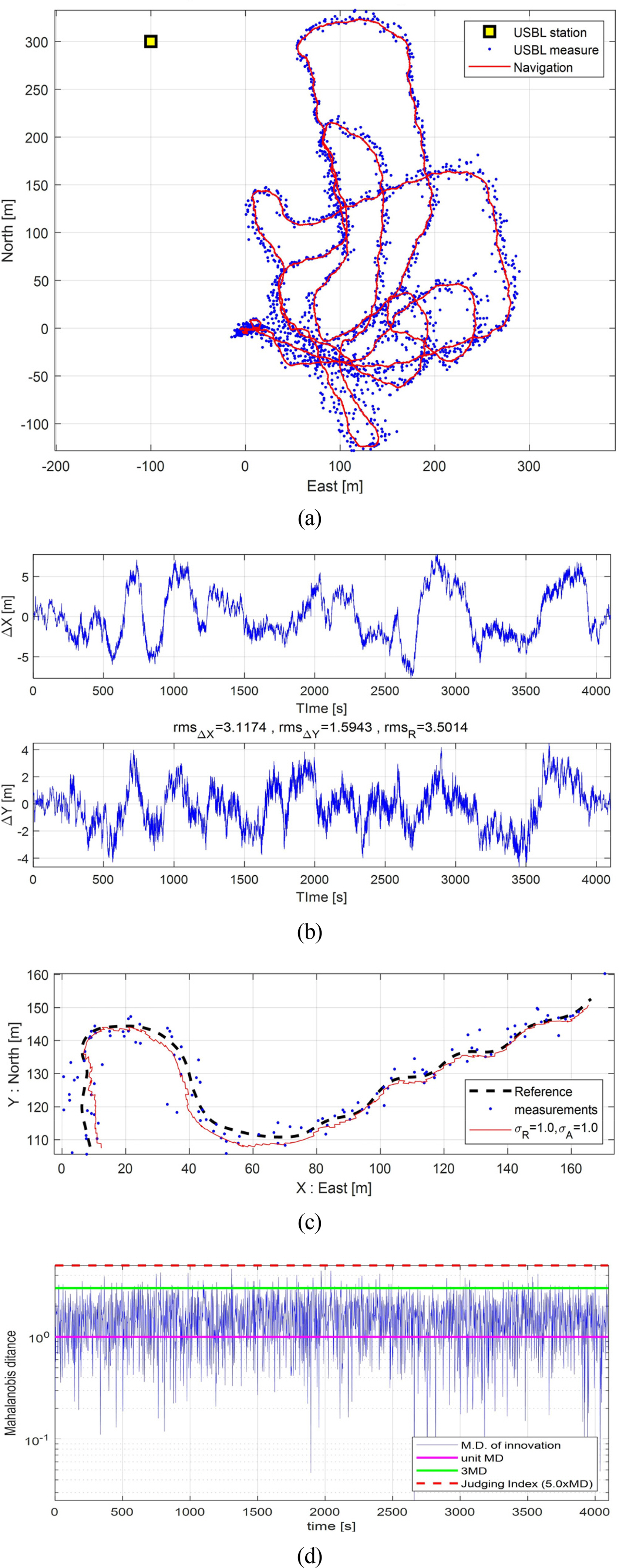
Simulation results of the navigation system using the uncorrelated error covariance model without outlier: (a) Trajectories of USBL measurements and estimated positions; (b) Navigation errors in the x- and y-positions; (c) The xy-plane trajectories: zoomed in for [3050, 3300] s; (d) Mahalanobis distance between the USBL measurements and the estimated positions
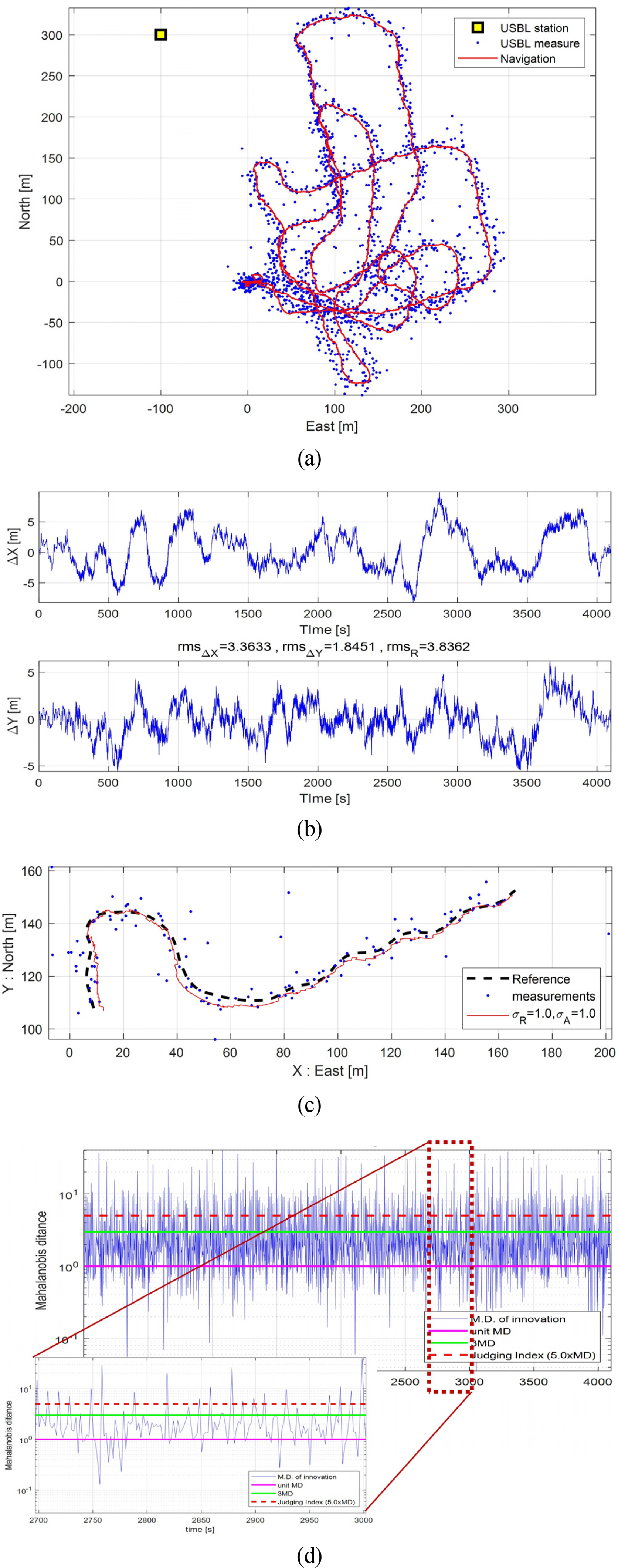
Simulation results of the navigation system using the uncorrelated error covariance model with outliers: (a) Trajectories of USBL measurements and estimated positions; (b) Navigation errors in the x- and y-positions; (c) The xy-plane trajectories: zoomed in for [3050, 3300] s; (d) Mahalanobis distance between the USBL measurements and the estimated positions
Figs. 10(d) and 11(d) show the MD for the errors between the USBL measurements and the estimated position of the navigation system. The vertical axis of these figures is on a logarithmic scale. The MD was calculated in three steps. After acquiring the error at each USBL measurement, the principal axis was obtained from the range and the relative azimuth angle between the estimated position and the USBL reference station. And then the MD was calculated by decomposing the error. In Figs. 10(d) and 11(d), the outlier judge level 5-σMD is indicated by the red dotted line. In the case of no outlier, the MD in Fig. 10(d) did not exceed the OJL over the whole time. In the case with the outliers, the MD frequently exceeded the OJL due to the outliers, as shown in Fig. 11(d). Although the differences between the estimated position and the USBL measurements were mostly within 4-σMD, the OJL was set as 5-σMD considering margin of the estimation error of the navigation system in these simulations. The navigation system stably detected and rejected the outliers larger than the criterion, as shown in the enlarged subplot in Fig. 11(d).
3.3 Performance of Outlier Rejection
In order to examine the outlier removal characteristics of the USBL-aided navigation system, the estimated positions of the navigation system with the uncorrelated error model was compared to those of the navigation system with a conventional error model. Fig. 12 (a) and (b) show the results of the estimated position of the two navigation systems in the xy-plane for the time [2350 2600] s, respectively. In these figures, the black dashed lines indicate the GPS trajectories of the AUV, that is, the true positions, the blue points represent the measured positions with the USBL, and the colored solid lines indicates the trajectories of the estimated positions for the case of four different OJLs. In Fig. 12(a), the estimated positions of the proposed method for the four levels of OJL between 3.5-σMD and 5-σMD were exactly the same, so the four colored solid lines were all overlapped on one trajectory. That is, the USBL-aided integrated navigation system with the USBL decorrelation model identified and removed the outliers in the same way even when the OJL was changed between 3.5-σMD and 5-σMD in the time period.

Estimated positions of the navigation system for the uncorrelated USBL model and the conventional model: (a) Proposed navigation; (b) Conventional navigation
In Fig 12(b), the estimated positions of the navigation system with conventional USBL error model were depicted with the colored solid lines, of which the OJL was 11, 16, 21, and 24m, respectively. It was shown that the estimated positions with the conventional error model were more affected by the outliers, which were not rejected when the OJL was specified larger. The smaller the OJL, the better the outliers were rejected. In such a conventional navigation system, it is required to make the OJL small in order to remove the outliers. However, if the OJL is not set larger than the intrinsic error bound of the USBL, the valid data of the USBL measurements will also be cut off.
The outlier reject characteristics were also reviewed, according to the OJL selection in the navigation system with the conventional error model of USBL. Because the total simulation time was 4,094 s, the number of the USBL measurements used in the simulation was 2,047. Among these signals, the number of the outliers included NOL was 410. The number of the outliers’ magnitude exceeding the OJL would be less than 410. Because the magnitude of the random outliers used in the simulation was uniformly distributed within the range of [0 Lmax (= 30)]m, the expected number of outliers can be expressed as Nexpected =NOL ×(1−OJL/Lmax ) in case of when there was no navigation error. The simulations were performed by adjusting the OJL for the navigation system with the conventional error model of USBL. Fig. 13 shows the estimated position errors with the conventional error model according to the OJL, as well as the number cut off the normal USBL signals needed for the navigation system.
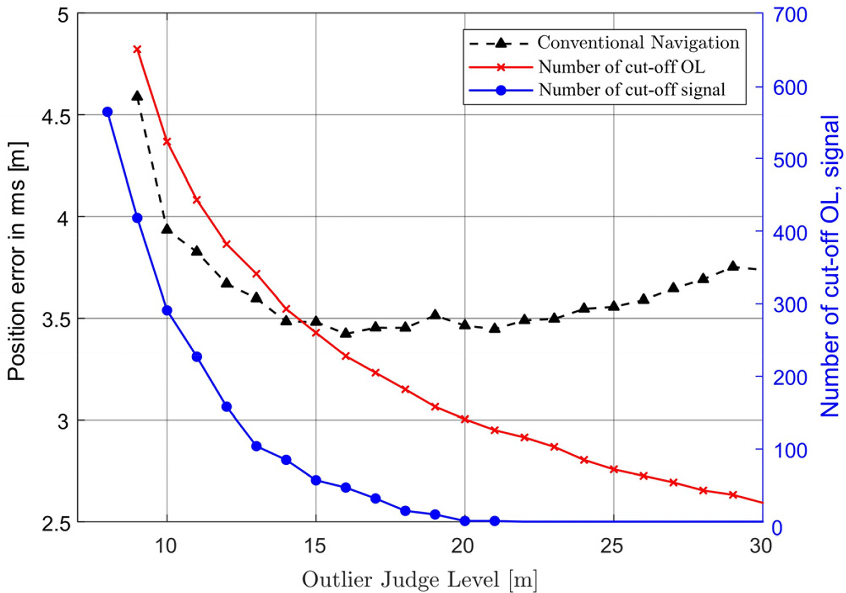
Estimation errors with a conventional USBL error model and the numbers of cut-off the OL data (including signals) and the signals only according to the OJL
The estimated position error showed a tendency to decrease as the OJL increased in the range of OJL ≤ 13 m, had minimum value in the range of 14 m ≤OJL ≤ 21 m, and gradually increased at OJL > 21 m. The OJL should be set larger than 21 m to design the navigation system so that the normal USBL signals were not cut off. Otherwise, some of the normal signals larger than the OJL would be discarded. When the OJL was 22 m, 116 signals were judged as outliers and discarded without losing normal signal. In this case, the expected number of outliers will be Nexpected = 109. Because the estimated position of the navigation system included errors, it is reasonable that the number of the blocked outliers differed from the expected value by approximately 6%. When the OJL was 16 m, the position estimation error was minimized, as shown in Fig. 13 and Table 3, while the number of the total blocked signal was 228. Among them, 47 normal USBL signals were blocked. The number of the blocked outliers in the simulation was 181, which differed approximately 5% from the expected number of 191. When the OJL was adjusted from 16 to 22 m, the blockage of the 47 normal signals was prevented. However, the 65 outliers were additionally considered as normal signals.

Numbers of cut-off outliers and normal signals with respect to the OJL for conventional navigation
Therefore, in the navigation system using the conventional error model of USBL, the loss of the normal USBL signals is inevitable for ensuring outlier rejection. When a large OJL is specified to avoid losing the normal signals of USBL, outliers within the OJL are identified as signals and adversely affects the navigation system. Conversely, when a small OJL is specified, some normal signals are lost, which also adversely affects the navigation system.
In contrast, the navigation system with the uncorrelated error model of USBL can designate the OJL according to the Mahalanobis distance, so it is possible to design a navigation system robust to outliers while preventing the loss of normal USBL signals. Fig. 14, similar as Fig. 13, shows the positioning errors of the proposed navigation system designed with OJL = 3.5-σMD and σR = 2.0 m, the number of the signals detected as outliers and cut-off (including the USBL signals), and the number of the cut-off normal USBL signals. In the figure, the horizontal axis represents the change of the OJL, of which the angular rms error of the USBL σψ is varying within the range [0.5 1.5]°. In the simulations, the rms error σψ was also related with the covariance of the noise vector in the navigation system. From the point of view of outlier rejection, a value larger σψ than 1.2 is required because the normal USBL signals were lost when it was designed with σψ ≤ 1.2°.
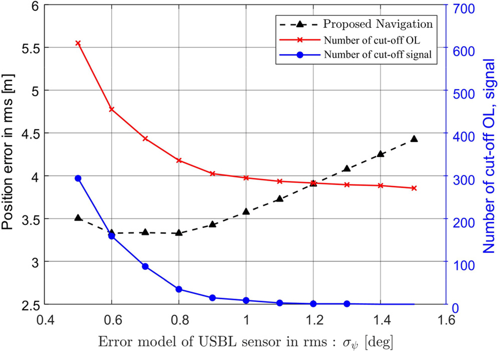
Estimation errors with the proposed USBL error model and the numbers of cut-off the OL data (including signals) and the signals only according to σψ = [0.5 1.5]° (fixed OJL = 3.5-σMD and σR = 2.0 m)
In Fig. 14 and Table 4, as σψ was set smaller, the number of the cut-off USBL signals increased. When σψ is set larger than 1.2, no signal was lost. In the range of σψ ≥ 0.8°, as the value of σψ increases, the number of the rejected outliers decreased, but the change was very small. In σψ < 0.8°, the number of the rejected outliers was independent of the level of σψ. When σψ = 1.2°, one normal signal was lost, and the 282 outliers were rejected. In this case, an equivalent OJL in the Euclidean space would be 9.3 m. From the simulations, the proposed method has shown better performance of outlier rejection than the conventional method. In these simulations, on the other hand, the measurement error model of the navigation system was related with the level of σψ of the OJL 3.5-σMD . When σψ was larger than 0.8°, the estimated position errors increased as σψ increases in the measurement error model of the system. So, it is required to designate a fixed value for σψ in the error covariance of the navigation system. Therefore, the navigation system with the uncorrelated model of USBL is more robust to outliers than the navigation system with a conventional error model of it.

Numbers of cut-off outliers and normal signals with respect to the OJL for the proposed navigation system
3.4 Blackout Response Characteristics
When the position measurement is not valid for a long time, the error of the navigation system increases in proportion to the blackout time. As the blackout time increases, the measured position of the USBL after the blackout might be significantly different from the estimated position of the navigation system. The outlier rejection method proposed in this paper can be applied when the navigation error is no larger than the order of the USBL position measurement error. Although it is beyond the scope of this article, the method of determining the integrity of the received USBL signal after a blackout requires the development of an algorithm that integrates the error characteristics of the navigation system and the intrinsic features of the USBL. In this study, after a blackout, the operation status of the navigation system was examined by applying a simple method of setting the outlier decision level to twice the existing OJL.
A simulation was performed on the position estimation of the navigation system with the error model of USBL. We supposed that when an AUV surveying under an ice-shelf received a new USBL measurement during a homing activity after performing its mission in a remote sea area where the USBL signal did not reach. It was assumed that a blackout occurred in [1000, 2400] s of the total simulation time of 4,094 s in the previous simulation. The rms errors of the radial and angular direction was σr = 1.0 m, σψ = 1.0°, respectively, and the outlier decision criterion was designed as 4-σMD in normal operation. In the simulation, the new reception of the USBL after the blackout occurred was considered a valid signal when the position deviation of Δx = x̃− x̂, i.e., the difference between the measured position and the estimated position, was within 8-σMD .
Fig. 15 shows the simulation results of the navigation system with the uncorrelated error model of USBL for the event in which a USBL blackout occurred. In Fig. 15(a), which presents the horizontal-plane trajectory, the estimated position denoted by the red solid line, the USBL measurements with outliers are shown as blue dots, and the USBLs that have not been received in the time zone of blackout are depicted in light gray. During the USBL blackout, the navigation system operated only with speed, attitude, and depth information. So, the AUV estimated the position that deviated from the true trajectory after 1,000 s of the blackout occurrence. The estimation error of position was up to about 81 m.

Simulation results of the USBL-aided navigation system including outliers and blackout occurred in [1000 2400] s: USBL signals with blackout and estimated trajectories; (b) Mahalanobis distance
When the USBL positioning signal was received again after 2,400 s, it was judged as a valid signal when and if the difference between the measured USBL position and the estimated position of the navigation system was within 8-σMD . So, even if a normal USBL signal is received, the measurement cannot be used immediately as the innovation of the navigation system under a large deviation Δx.
As shown in Fig. 15(b), the MD between the measured position of USBL and the estimated position at 2,400 s was 47.1-σMD, exceeding the threshold level of 8-σMD . So, the AUV judged this signal as an outlier and did not use it as an innovation signal for the navigation system. Even when the normal USBL position measurement data were subsequently received, the navigation system continued to discard the USBL position measurement, because the deviation Δx exceeded the OJL. At 2,540 s, when the position error was within the range of 8-σMD, the navigation system used the USBL position measurement signal to update the error covariance, and the estimation error of the navigation system rapidly decreased and converged to the true position within 10 seconds. A further study on the integrity judgment reflecting the USBL positioning data received after a blackout and the navigation error is required.
4. Conclusions
This paper proposes a USBL-aided underwater navigation system with the uncorrelated error model of USBL, which can be applied to survey under Antarctic ice-shelf or missions in shallow water. The Mahalanobis distance (MD) and principal components (PC) of the USBL measurements in the horizontal plane were analyzed, of which the magnitude of the error and the direction of the principal axis of the error distribution varies according to relative position and distance between the reference station, typically USBL transceiver, and an AUV. Simulations of the navigation system were performed by synthesizing the measured data and the numerically generated data. A measured position dataset of the USBL were generated by adding the intrinsic noise of a USBL and the random outliers in magnitude and direction to the relative position between the GPS position and a reference station of the USBL. The proposed method can effectively reject the outliers without loss of the USBL signals by decorrelating the error covariance of the radial direction and its orthogonal direction of the USBL in the horizontal plane, and judging whether the USBL measurement is outlier based on the Mahalanobis distance. The simulation results indicated that the navigation system with the uncorrelated error model of USBL can reject outliers more robustly than the navigation system with a conventional error model of USBL. It was also illustrated that the estimation error of the navigation system may be reduced by applying the USBL measurement received after a blackout. The outliers of USBL would be apt to change in frequency and/or magnitude, depending on the sea conditions such as changes in water temperature and salinity. Therefore, it is necessary to adjust the outlier decision level accordingly to match the environmental conditions of the operating area of the AUV through field experiments at sea in the future. Further study is additionally required to analyze the integrity of the new measurement of the USBL after a long blackout and the convergence of the estimation error of the navigation system to the true position.
Notes
This article is based on a thesis presented at the Korean Association of Ocean Science and Technology Societies (KAOSTS) Joint Symposium and is a detailed and expanded version of it (Lee et al., 2022).
No potential conflict of interest relevant to this article was reported.
This study was conducted with the support of the “Development of core technologies of underwater robot ICT for polar under-ice-shelf exploration and remote monitoring (4/5)” and the Korea Coast Guard, as a key technology project of the Korea Research Institute of Ships and Ocean Engineering. These findings are a part of the ongoing research results of the “Development of AUV fleet and its operation system for maritime search (2/5).”