Trajectory Tracking Performance Analysis of Underwater Manipulator for Autonomous Manipulation
Article information

Abstract
In this study, the end-effector tracking performance of a manipulator installed on a remotely operated vehicle (ROV) for autonomous underwater intervention is verified. The underwater manipulator is an ARM 7E MINI model produced by the ECA group, which consists of six joints and one gripper. Of the six joints of the manipulator, two are revolute joints and the other four are prismatic joints. Velocity control is used to control the manipulator with forward and inverse kinematics. When the manipulator approaches a target object, it is difficult for the ROV to maintain its position and posture, owing to various disturbances, such as the variation in both the center of mass and the reaction force resulting from the manipulator motion. Therefore, it is necessary to compensate for the influences and ensure the relative distance to the object. Simulations and experiments are performed to track the trajectory of a virtual object, and the tracking performance is verified from the results.
1. Introduction
A manipulator can perform various tasks within a certain work space, and is used in a diverse range of applications in manufacturing and research. When a manipulator is fixed at a specific location to perform tasks, problems such as the constraints of the work space and the occurrence of singularity are encountered. To address these problems, a manipulator is mounted on a vehicle to perform mobile manipulation to interact with a target object. A robot with wheels and unmanned aerial vehicle such as drone are equipped with manipulators to perform the work (Kim et al., 2019; Korpela et al. 2012). Research is underway to carry out the work by installing a manipulator on a remotily operated vehicle (ROV) or an autonomy underwater vehicle operated not only on the ground and in the air but also on the ocean (Ribas et al. 2012, Kang et al. 2017).
Underwater manipulators installed on underwater vehicles have the following considerable differences from on-shore industrial manipulators: (1) the former structures can withstand deep-sea environments, (2) they are small and lightweight considering the nature of underwater vehicles, and (3) their underwater intervention is diverse and complex (Ura and Takakawa, 1994/2015).
Since the deep sea environment is unique in that the pressure increases with the depth, the actuator of a manipulator must be manufactured to be pressure resistant and with a pressure equalization method capable of withstanding the pressure of the working depth. Owing to the characteristics of an underwater vehicle, there are constraints on the space and weight; therefore, its manipulator should be small and lightweight. In addition, an underwater manipulator must be able to respond to various operational scenarios occurring in a deep-sea environment; in comparison, the objective of an on-shore industrial manipulator is to perform a predetermined task repeatedly and accurately in a certain space. Therefore, an underwater manipulator is a man–machine system that requires operator judgment or manipulation of the manipulator control system. In this regard, studies have been conducted recently on autonomous manipulators that plan and execute intervention with simple instructions from an operator for pre-defined specific tasks.
The Korea Research Institute of Ship & Ocean Engineering (KRISO) has developed an underwater autonomous robot platform equipped with a manipulator on a remotely operated vehicle (ROV). This underwater robot can automatically perform a series of tasks in which it recognizes the position of a target object, approaches the object, and grasps the object using a manipulator (Yeu et al., 2019).
In this study, the position tracking performance of the manipulator, ECA ARM 7E Mini model, is analyzed for autonomous intervention of underwater robots. For realizing the autonomous manipulation of underwater robots, forward and inverse kinematics are used to control the manipulator. The distance between an underwater robot body and the end-effector is obtained using forward kinematics, to determine the position of the end-effector according to the manipulator joint angle. In addition, the value of the joint angle to reach a target object for autonomous manipulation is calculated using inverse kinematics, which determines the position of the joint angle of the manipulator according to the position of the end-effector in arbitrary Cartesian coordinates. The ECA ARM 7E Mini manipulator consists of six degrees of freedom and one end-effector. Of the six joints, four are prismatic joints and two are revolute joints. The output of a prismatic joint of the manipulator in length units is converted into angular units using the kinematic correlation, and this was utilized in the calculation of the forward and inverse kinematics of the manipulator and for the velocity control algorithm.
When an underwater robot performs autonomous manipulation, disturbances, such as the reaction force from the manipulator operation, cable impacts, and external fluid force, arise. If these disturbances are not appropriately compensated owing to the lack of control performance or other reasons, the position and posture of the underwater robot will change, and a target point of the manipulator will vary continuously. For smooth autonomous manipulation by compensating for the constantly varying distance and the direction between the end-effector and a target object, an algorithm that allows the end-effector to tack the target object is developed, and its performance is demonstrated.
The structure of this paper is as follows. Chapter 2 introduces the developed ROV for autonomous underwater manipulation. It also describes the manipulator specifications, kinematics, and inverse kinematics information. In addition, it presents the conversion method of the output information of the prismatic joints of the manipulator into angular information as well as the algorithm allowing the end-effector to track a target point. Chapter 3 presents the verification of the end-effector tracking algorithm using simulation. Chapter 4 describes the demonstration of the algorithm, verified by the simulation, using a manipulator installed on an underwater robot and analyzes the result of the underwater tracking of a target object. Chapter 5 presents the conclusion.
2. ROV for Autonomous Underwater Manipulation
2.1 Underwater Robot Platform
The underwater robot developed by KRISO for autonomous underwater manipulation is displayed in Fig. 1. The underwater robot for autonomous manipulation is primarily divided into upper and lower parts; the upper part is equipped with a thruster, electronic parts, and a buoyancy module, and the lower part comprises an ECA underwater manipulator ARM 7E Mini and related accessories. When operating for investigation and exploration purposes, the ROV function can be performed with the upper part alone, whereas for autonomous underwater manipulation, as presented in Fig. 1, autonomous manipulation is performed with both the upper and lower parts. The underwater robot measures the velocity and posture using an installed inertia measurement unit (IMU), a Doppler velocity log (DVL), and a depth sensor, and the position of the underwater robot is determined by these measurements. Subsequently, a target object and its position are identified using a camera and an underwater laser scanner.
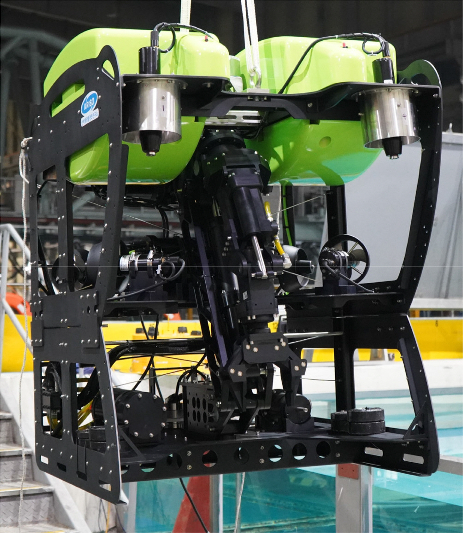
Underwater robot with ECA ARM 7E Mini
2.2 Underwater Manipulator
The ARM 7E Mini model (Fig. 2), a manipulator for autonomous manipulation installed on the above underwater robot, is a commercial product that can operate up to 300 m underwater. Its weight on the ground and underwater weight are 50.8 kg, and 33.8 kg. respectively. Of the six joints of the ARM 7E Mini, four are prismatic joints and two are revolute joints.
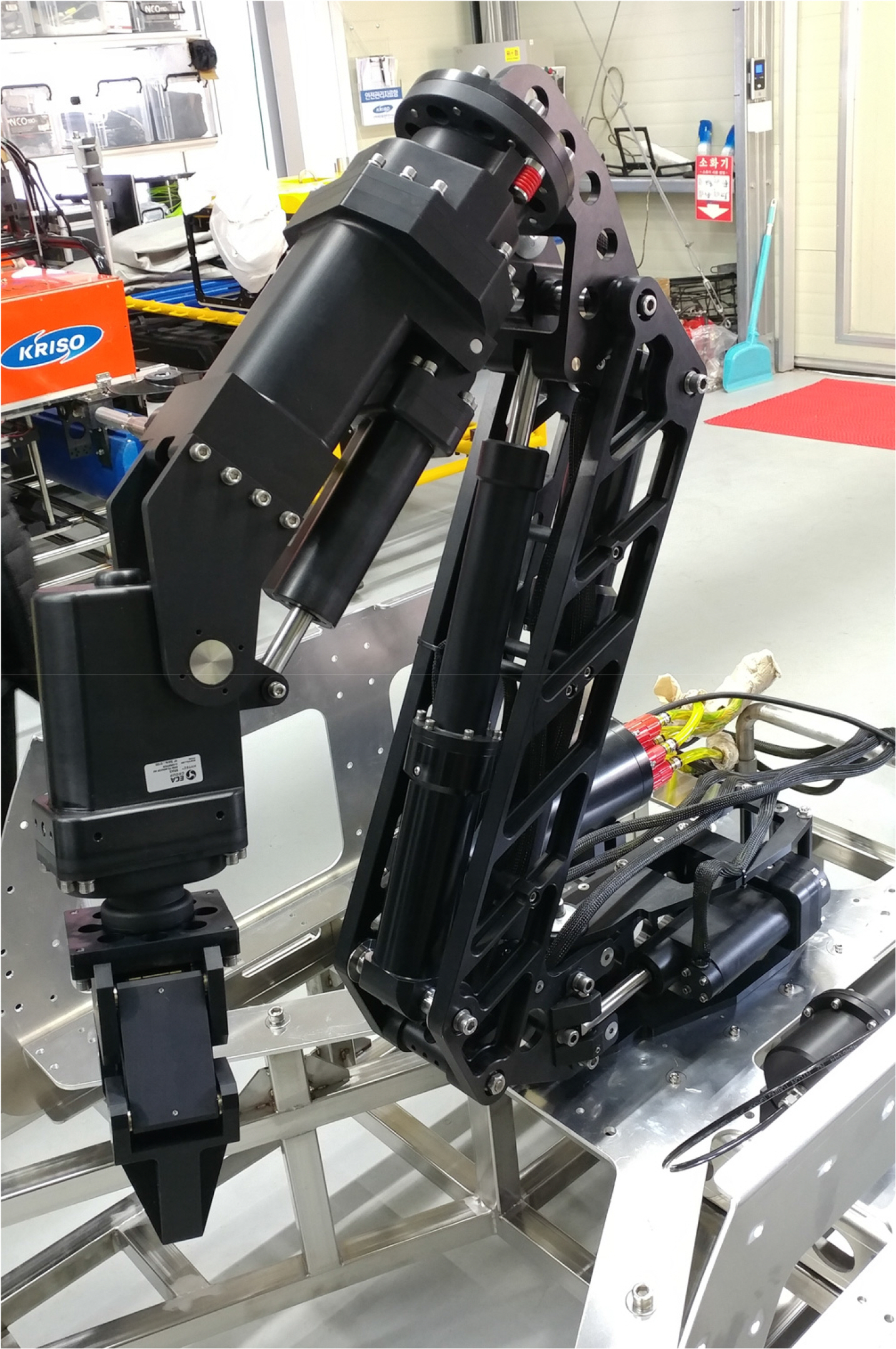
ECA ARM 7E Mini
2.2.1 Kinematic information
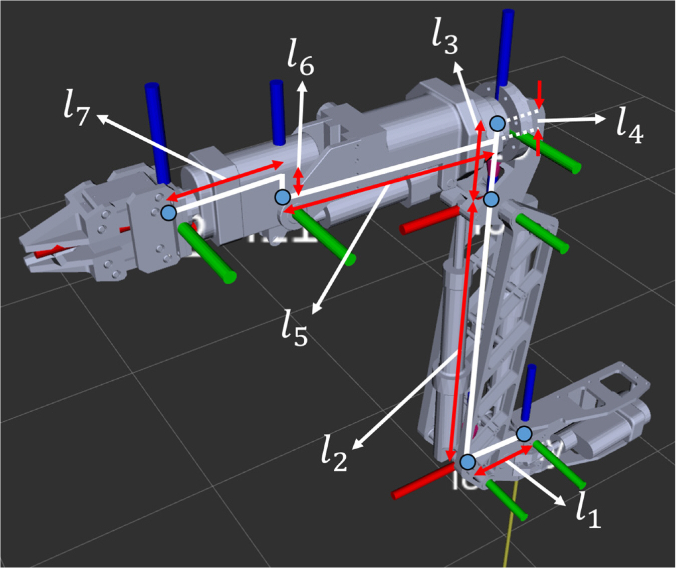
The output of the of a prismatic joint of the manipulator in length units was converted to angular units using the kinematic correlation, and this was applied to the forward and inverse kinematics of the manipulator. For the control of the manipulator, it was operated at 10 Hz, and the control input of the manipulator was the joint velocity. Table 1 summarizes the range of motion of each joint of the ECA ARM 7E Mini and the link length. In addition, when all joint angles are 0°, the length information of the link and the shape of the manipulator are as presented in Fig. 3, and the information of the joint coordinates and the rotational axis of the joints is as depicted in Fig. 4.
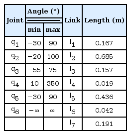
Joint angle and link length information
Links of ECA ARM 7E Mini
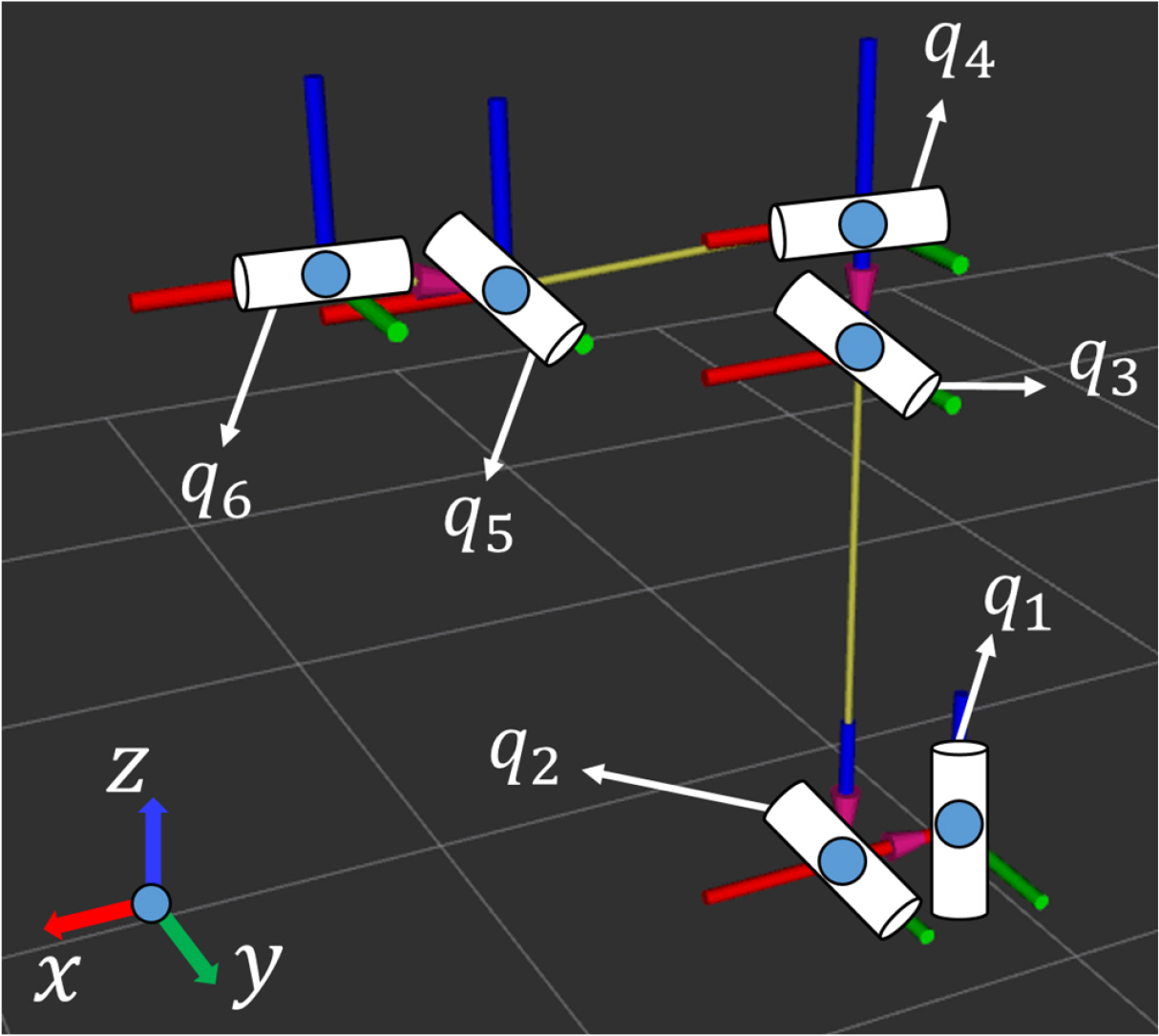
Joint axes of the ECA ARM 7E Mini
2.2.2 Prismatic joint–revolute joint transformation
Although the output of the manipulator is obtained in terms of the prismatic joints, the kinematics is described using the revolute joints, instead of the prismatic joints. This is because the manipulator is designed to rotate around the axis as a prismatic joint changes, so that it is easier to describe the kinematics with the revolute joints compared to when using the prismatic joints.
To control the manipulator based on the inverse kinematics, the position and velocity output of a prismatic joint are converted into angle and angular velocity, respectively. Here, the prismatic joints are denoted as q1, q2, q3, and q5, and the revolute joints are referred as q4 and q6. To convert the length outputs of the four prismatic joints into rotational angles, we examine the relationship between a length output and a rotational angle.
The relationship between the length output and rotational angle for the second joint is as presented in Fig. 5. In the red triangle, the lengths of the two sides, which are constants determined by the kinematic characteristics, are set as b2 and c2, respectively; the angle between the two sides is q́2, and the length of the other side is set as d2. Here, the included angle, q́2, is specified according to the manipulator length output, d2. For using a joint angle as specified in Table 1 and Figs. 3 and 4, a constant, qoffset,2, is added to the specified q́2 to obtain the joint angle, q2.
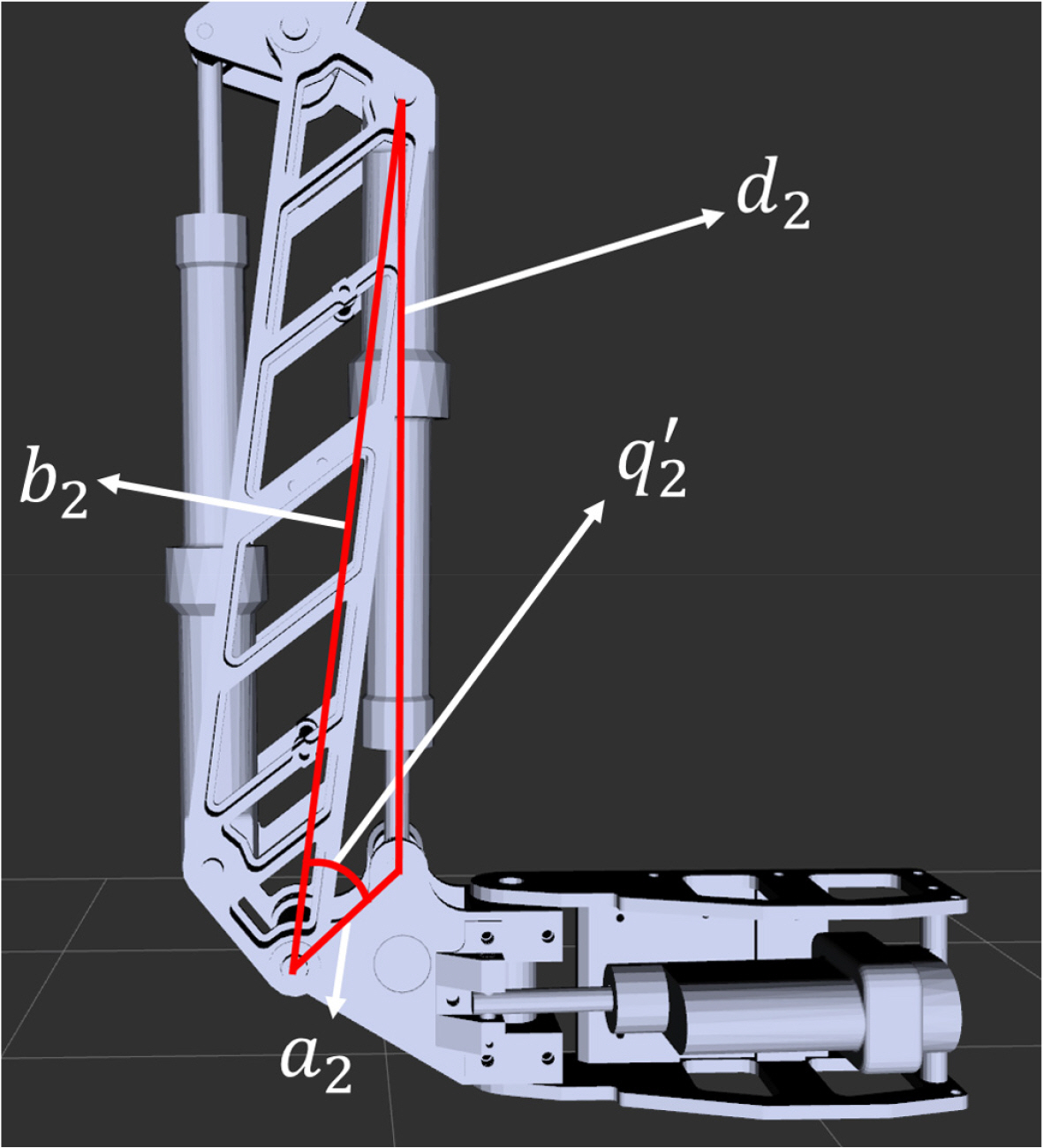
Configuration of second prismatic joint d2, revolute joint q́2, and constant b2 and c2
Similarly, for joints i = 1,2,3,5, which are the length outputs, position variable di, outputs of the prismatic joints, angular variable q́i of the revolute joints, and constants ai and bi corresponding to the two sides of the triangle, the relationship between di and q́i is described in Eq. (1) by the second cosine law.
Arranging Eq. (1) with respect to q, we obtain Eq. (2), and the angle of each joint output from the manipulator can be obtained. Here, the range of the variable, di, is typically within the range that satisfies the condition of a triangular formation with bi and ci. Therefore, under the condition that the sum of the lengths of two sides is greater than the length of the other side,
For the conversion into the joint angle as specified in Table 1 and Figs. 3 and 4,qi is calculated by adding qoffset,i to q́i as expressed in Eq. (3). Here, qoffset,i is a constant determined according to the kinematic characteristics and kinematic description of each joint
In addition, the relationship between the velocity variable, ḋ, of a prismatic joint and the angular velocity variable, q̇, of a revolute joint can be obtained by differentiating Eq. (1).
Substituting Eq. (2) into Eq. (4), the angular velocity output from the manipulator is as follows.
2.3. Control Algorithm
To control the manipulator to reach a desired position, the position of the target joint angle for a given Cartesian position of the end-effector needs to be obtained. However, since a general method for solving inverse kinematics by analytical methods has not been identified, the inverse kinematics is solved using an inverse Jacobian matrix, a numerical method. q̇d is the target input velocity vector of the manipulator, ẋd is the target velocity vector of the end-effector in the rectangular coordinate system, and J is a Jacobian matrix that linearizes the relationship between the end-effector velocity vector and the manipulator joint velocity vector. Therefore, Eq. (6) can be obtained using the relationship of q̇d, J, and ẋd.
To improve the error in the joint velocity input resulting from the numerical integration in Eq. (6) and the tracking performance, closed loop inverse kinematics (Colume and Torras, 2014) is used to calculate the velocity input value of the manipulator, as expressed in Eq. (7).
q is the angle vector of the current joint angle fed back from the manipulator, qd is the target angle vector of the joint angle calculated based on inverse kinematics, and k is the gain value for the joint angle position error.
2.4. Tracking Algorithm
The position of an underwater robot changes under an arbitrary external force generated when the underwater robot performs autonomous manipulation. In this case, since the target for the interaction with the manipulator changes its position with reference to the underwater robot, the manipulator needs to continuously track the target. When the position vector of the end-effector is x in the Cartesian coordinate system, ẋd is defined as Eq. (8), the end-effector can continuously track the position vector, xobj of the object to interact with.
If ẋd is set as in Eq. (8), the manipulator moves at velocity V in the direction of the target object in the Cartesian coordinate system.
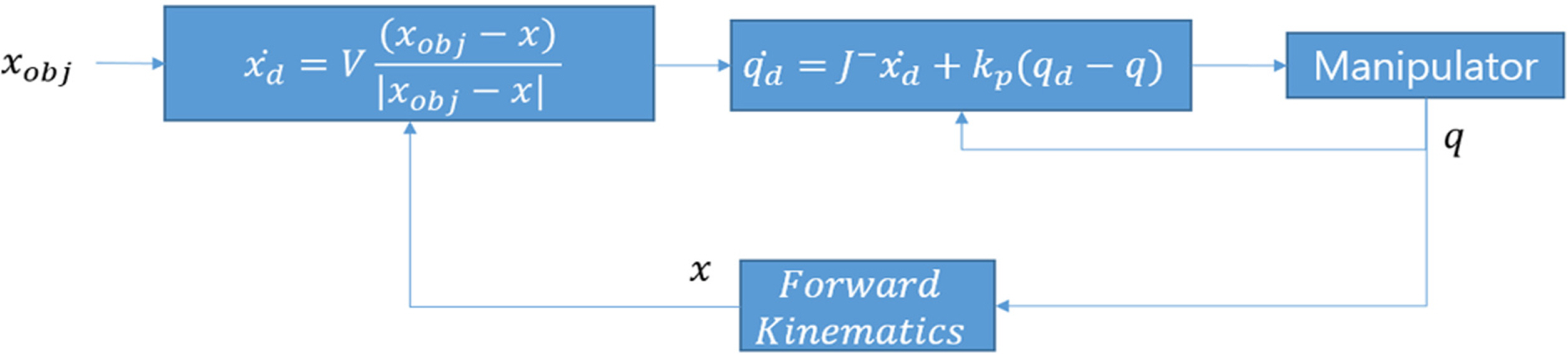
Here, dt is defined as the time required for one control loop and vmax is defined as the maximum velocity that the end-effector requires for each control loop. When the velocity of the manipulator installed on the underwater robot is high, the subsequent fluid impact and an abrupt movement of the center of mass can adversely affect the position control of the underwater robot. Therefore, the movement velocity, V, of the end-effector is given as in Eq. (8). If the difference between the position of the target object and the end-effector is greater than vmax/dt, the velocity of the end-effector is set as vmax . If the difference is less than vmax/dt, it is set as |xobj – x|dt, proportional to the position difference between the object and the end-effector. Therefore, when the end-effector tracks the target object, it is moved with vmax at maximum. The controller of the manipulator is configured, as displayed in Fig. 6, using the inverse and forward kinematics. As presented in Fig. 6, the angle output, q, of a joint angle is obtained, and using the forward kinematics, the end-effector position, x, is obtained in the Cartesian coordinates system.
Control loop of manipulator
3. Tracking Algorithm Simulation
Prior to verifying the tracking performance of the manipulator, we aimed to verify the performance of the tracking algorithm by simulation. For the simulation environment, the open dynamics engine (ODE) of the open-source robotics foundation (OSRF) in Gazebo 7.15.0. ver. is used (Fig. 7). An ECA ARM 7E Mini model was fixed in the bottom of the Gazebo simulation environment, and the simulation was performed. Unlike the actual manipulator model, all the joints were assumed to be revolute joints in the simulation performance.
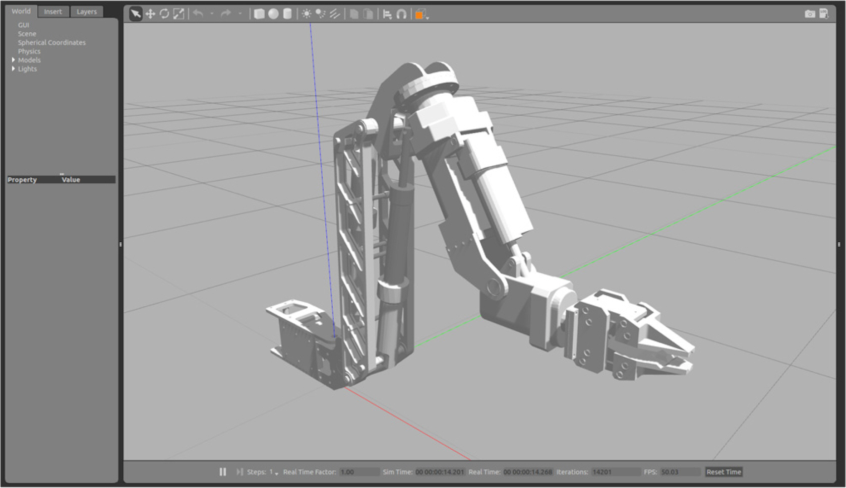
Gazebo simulation with the ECA ARM 7E Mini
3.1 Linear Tracking Simulation
For the linear tracking simulation, from the initial position of the end-effector, for tracking the trajectory of a point moving to a target (X = 0.2 m, Y = 0 m, Z = 0 m) positioned on a horizontal line, as depicted in Fig. 8, the trajectory of a point moving to a target (X = 0.1 m, Y = 0 m, Z = −0.2 m) positioned diagonally, as presented in Fig. 9, was determined.
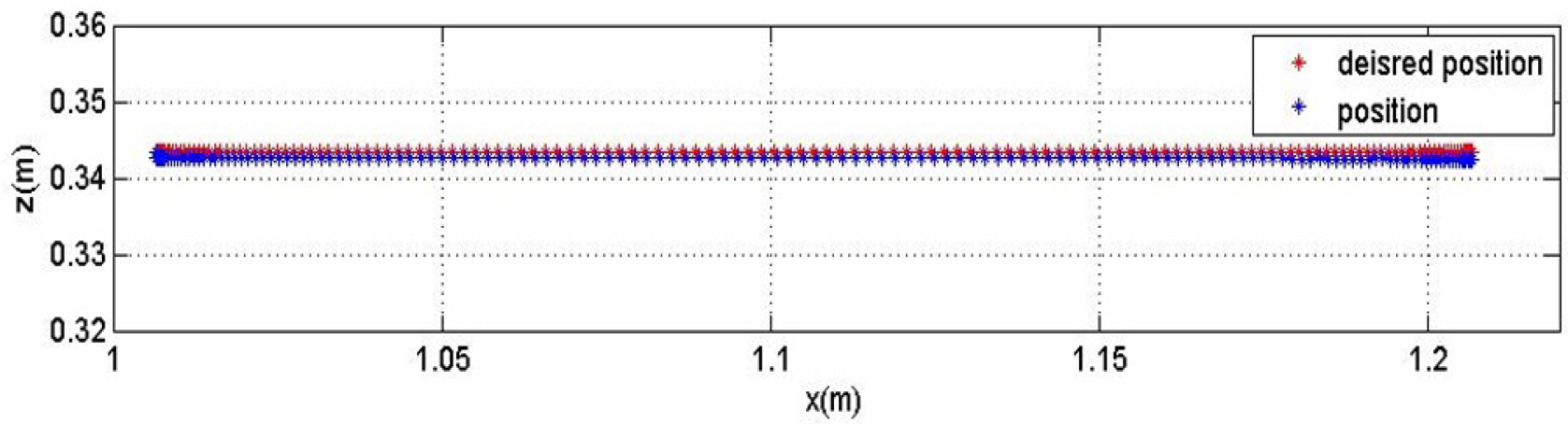
End-effector trajectory of a horizontal movement obtained from the simulation

End-effector trajectory of a diagonal movement obtained from the simulation
The plots of the end-effector position and the position error of the horizontal tracking presented in Fig. 8 and of the diagonal tracking in Fig. 9 are indicated in Figs. 10 and 11, respectively. The two figures in the upper part of Fig. 10 display the position and position errors in the X and Z directions, respectively. In the X and Z directions, the maximum position errors are approximately 3.3 mm and 1 mm or less, respectively. After the movement, the position error in the steady state is 0.1 mm in the X direction and 0.8 mm in the Z direction. The figures in the upper part of Fig. 11 display the position and position errors in the X direction and Z directions. The maximum position error in the X direction is approximately 2.3 mm, and it is 2 mm in the Z direction. After the movement, the position error in the steady state is 0.1 mm in the X direction and 0.8 mm in the Z direction. After completing the movement in both the horizontal and vertical directions, the error in the Z direction is greater than that in the X direction. As the manipulator moves further away, the length of the moment arm increases at a particular gravity, and the torque loaded on the specific joint increases. With the increase in the torque, the position error of the joint increases. However, as expressed in Eq. (7), when there is an error in qd, the target position of the joint, and q, the joint position. When the velocity input increases to compensate the error, the error becomes less than 1 mm in the steady state in the Z-direction. During the movement, the end-effector velocity is determined in proportion to the position and error of the point to be tracked by the manipulator, as written in Eq. (9). Accordingly, it can be estimated that a position error will occur in proportion to the acceleration of the object to be tracked, which can be seen by comparing the position error variation in the X direction with acceleration and that in the Z direction without acceleration. Compared to the X direction position error graph, in the Z direction position error graph, since there is no acceleration of the object, we can see that the position error is small.
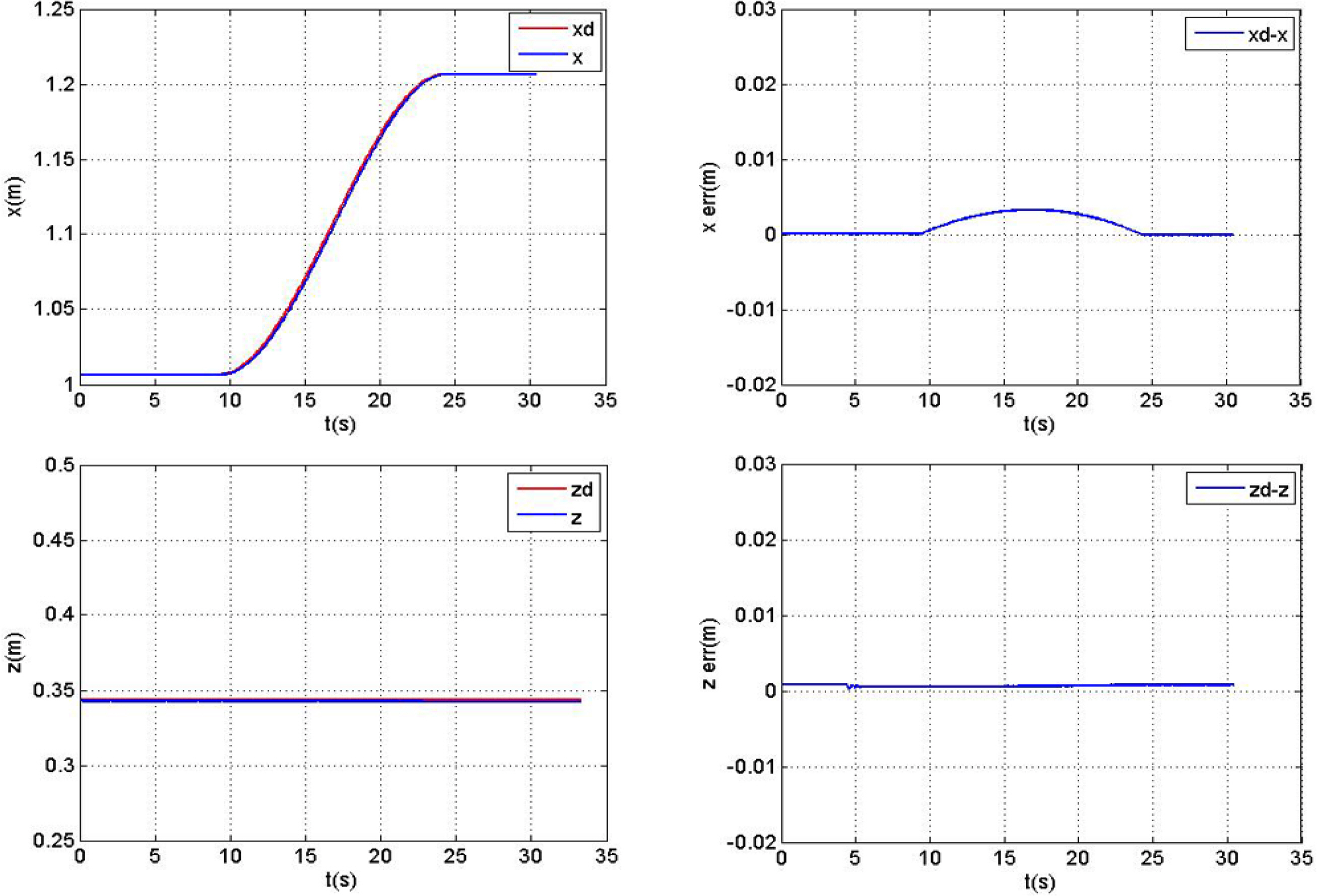
Position and error for a horizontal movement obtained from the simulation
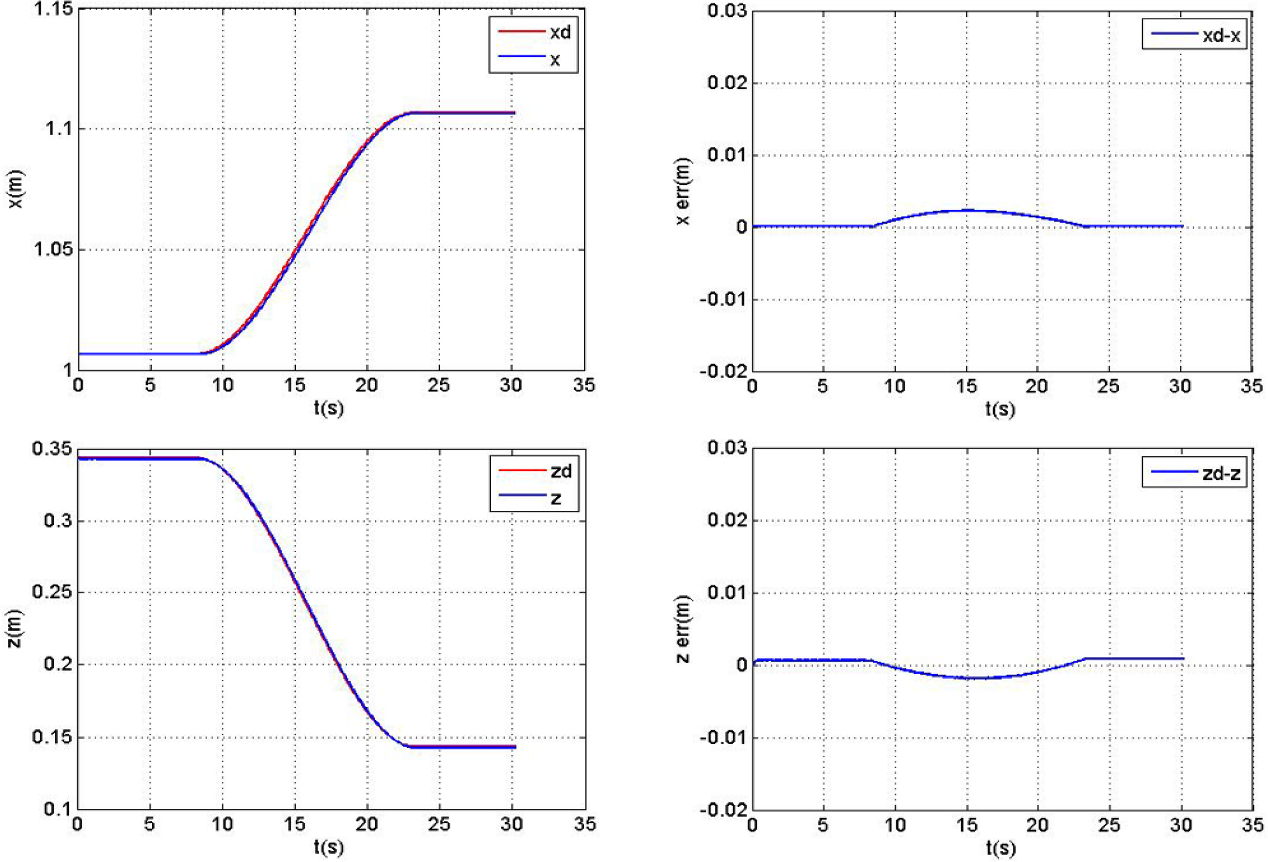
Position and error for a diagonal movement obtained from the simulation
3.2 Circular Tracking Simulation
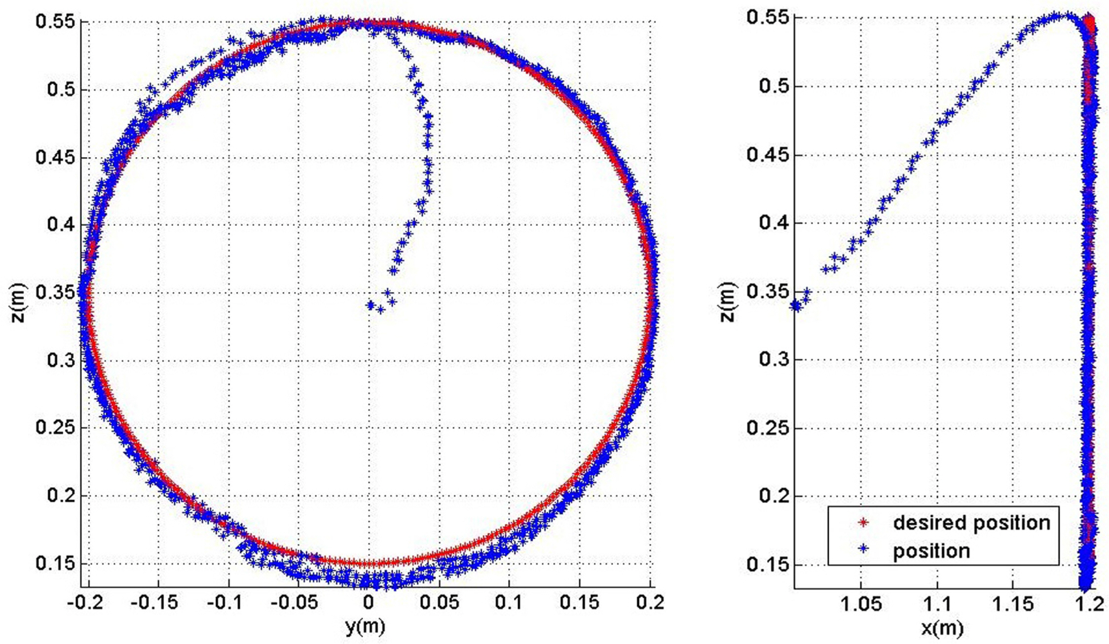
In this section, we present the analysis of the simulation in which the end-effector tracks the position of a point moving along the trajectory of a circle over time. A circular tracking simulation was performed (Fig. 12) to track the position of a target object moving along a circle with a radius of 20 cm, 20 cm away from the end-effector in the X direction
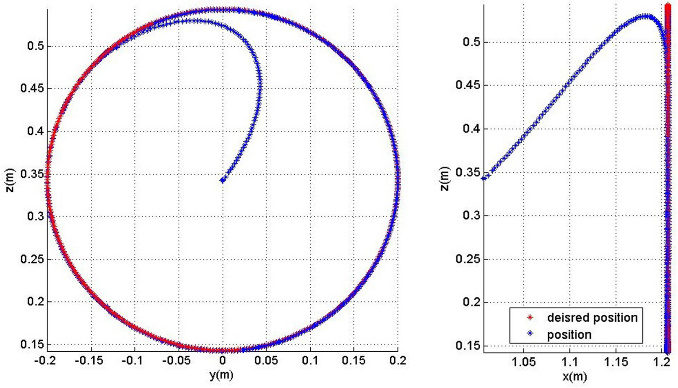
End-effector trajectory for a circular movement obtained from the simulation
In Fig. 12, the red dot is the trace of the target object moving along the circle, and the blue dot is the trace of the end-effector position. At the beginning of the simulation, it can be seen that the manipulator end-effector moves to the front and the upper side where the target object exists. It then continues to track the path of the moving point after the target object position and end-effector are sufficiently close. Fig. 13 displays the position and position error graph, in which the left is the position graph, and the right is a position error graph. As soon as the movement starts, it can be noted that the blue line, which is the end-effector position, moves to the red line, which is the target position. Moreover, the red line continuously tracks, after the end-effector reaches the position near the moving point. In the position error graph, it can be seen that the position error decreases rapidly at the beginning of the operation, and over time, it tracks with an error of up to 5 mm in the Y and Z directions.

Position and error for a circular movement obtained from the simulation
4. Tracking Performance Demonstration Experiment
This chapter describes the demonstration of the position tracking performance of the ECA ARM 7E Mini Manipulator by experiments. By applying the control and tracking algorithms used in the simulations, as discussed in Chapter 3, to an actual manipulator, we conduct experiments in which the end-effector performs linear tracking and circular tracking. Finally, the manipulator is installed on an underwater robot, and an underwater tracking experiment of a target object is performed.
4.1 Linear Tracking Experiment
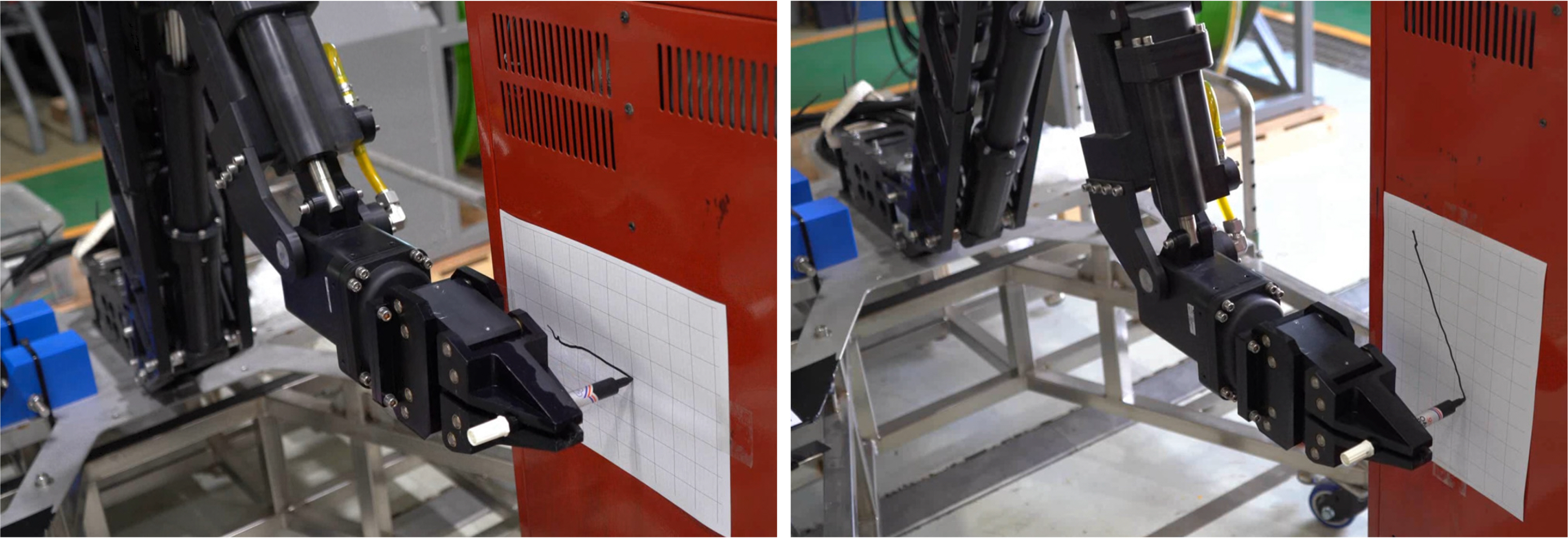
To verify the linear position tracking performance of the manipulator end-effector, an experiment was conducted as follows. After a grid paper was attached to a flat surface perpendicular to the Y = axis, the end-effector was directed to grasp a pen. After keeping the pen and grid paper in contact at the initial position of the end-effector, horizontal tracking (X = 0.2 m, Y = 0 m, Z = 0 m) and diagonal tracking (X = 0.1 m, Y = 0 m, Z = −0.2 m) experiments which were simulated as discussed in Chapter 3 were performed. Figs. 15 and 16 present the graph of the linear movement of the end-effector superimposed on the grid paper drawn with a pen. Here, the red dots are the target positions of the end-effector in Cartesian coordinates. The blue dots are the current position of the end-effector calculated using the forward kinematics based on the joint angle fed back from the manipulator. Here, there are parts where the initial control is unstable owing to the friction when the joint angle of the manipulator moves after stopping. In addition, there are errors from the kinematic modeling and tilting of the floor. However, overall, it can be confirmed that the trajectory of the end-effector and the trajectory drawn by the pen are similar.
Horizontal movement trajectory of the end-effector obtained from the experiment (Red: desired, Blue: measured, Black: drawn)

Diagonal movement trajectory of the end-effector obtained from the experiment (Red: desired, Blue: measured, Black: drawn)
The results of the horizontal tracking (Fig. 17) and diagonal tracking (Fig. 18) performed by the end-effector are examined according to the movement time. The upper left graph is a plot of the X -direction target position of the end-effector and the current position, and the upper right graph is the X-direction position error plot. In the horizontal and diagonal tracking, when the manipulator starts to move for the first time, errors of up to 7 mm and 4 mm occur in the X -direction, respectively, and errors of less than 1 mm occur in the steady state after the manipulator completes the movement. The lower left graph displays the Z-direction target position of the end-effector and the current position, and the lower right graph presents the Z-direction position error. In the horizontal and diagonal tracking, during the movement of the end-effector, errors of up to 12 mm and 13 mm occur, respectively, and errors of approximately 4 mm and 1 mm occur, respectively, in the steady state after the manipulator arrives at the target point. It can be seen from the position error graph that the tracking error is relatively large in the low-velocity sections (10–15 s, 20–25 s) during the movement of the manipulator. The tracking error can be inferred as a decrease in the performance of the tracking of the position of the joint actuator when the joint is driven at a low velocity. Under the decreased tracking performance due to the low velocity, the position tracking performance of the joint angle is further deteriorated by the load, which emerges as a position error in the form of a deflection. Therefore, it can be confirmed that the position tracking error is larger than that obtained from the simulation.
Position and error for a horizontal movement obtained by the experiment
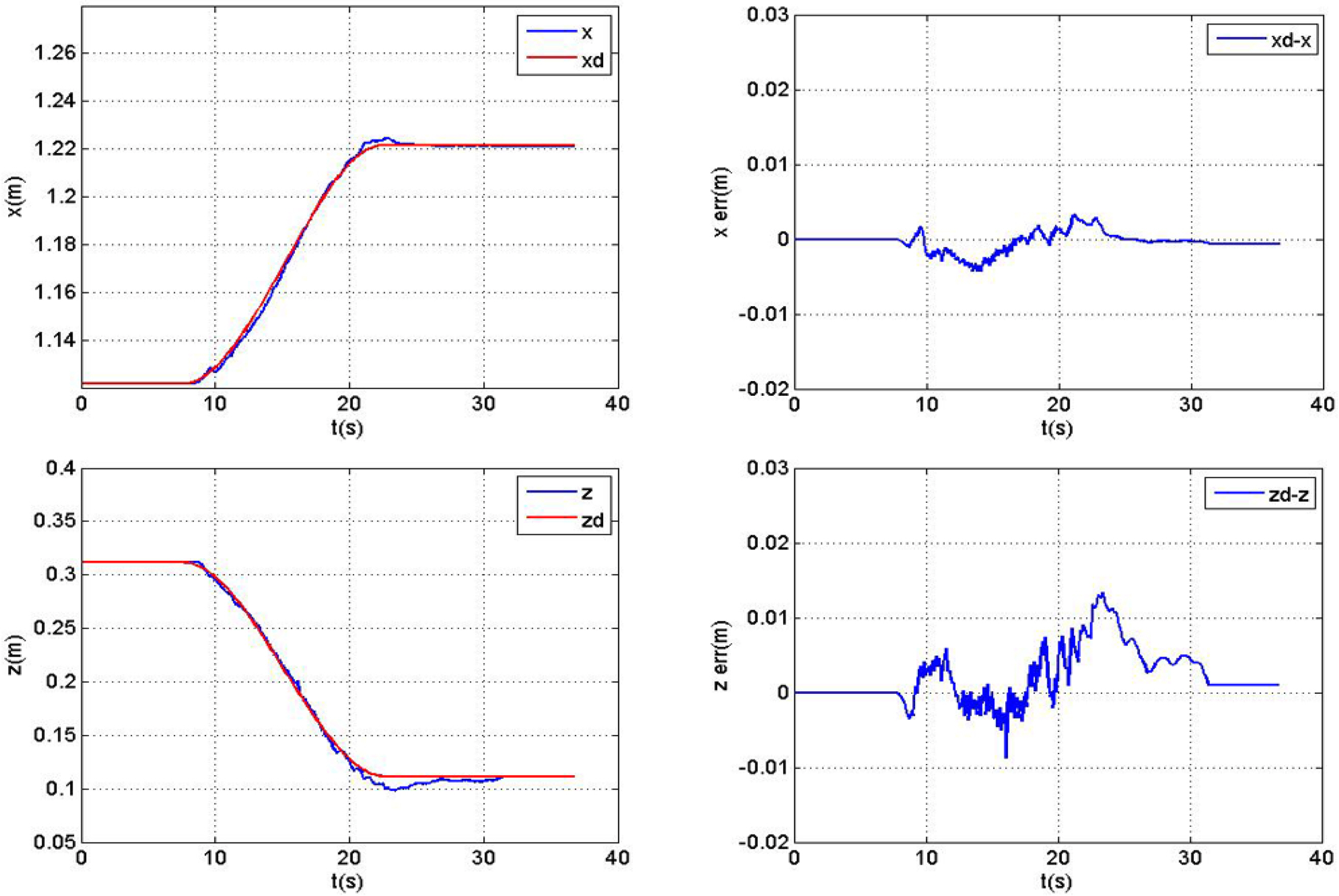
Position and error for a diagonal movement obtained by the experimen
4.2 Circular Tracking Performance Demonstration
Here, we present the experimental demonstration of the circular tracking performance verification, described using simulation in Chapter 3.2. The results of the experiment in which the end-effector of the manipulator tracks a continuously moving object in a circular motion are examined in this section. The left figure of Fig. 19 illustrates the manipulator tracking a virtual purple sphere, and it shows the shape of the manipulator based on the joint angle fed back from the manipulator. The picture on the left is that of the manipulator viewed from the side when the manipulator tracks the virtual sphere.
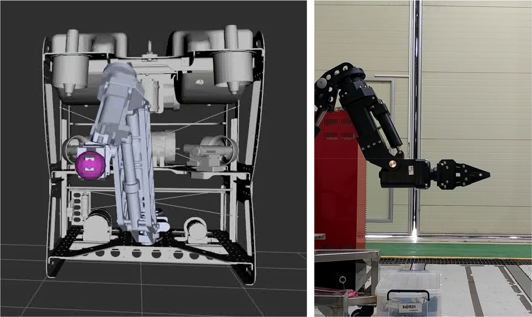
Experimental tracking of a virtual sphere by the end-effector
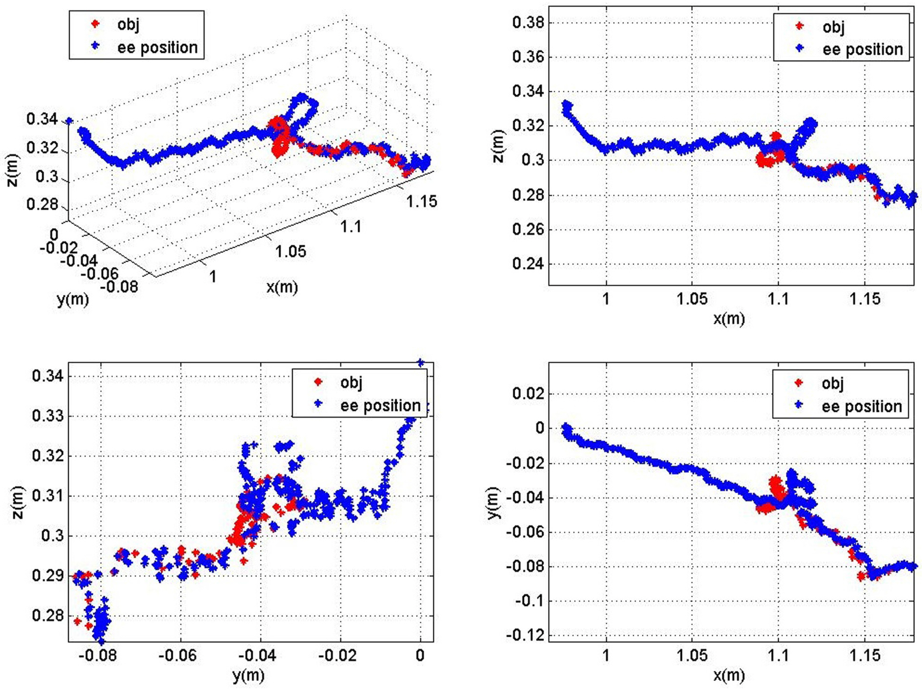
Fig. 20 displays a graph showing the trajectory of the end-effector tracking a virtual sphere moving in a circular motion in the Cartesian coordinate system. The left figure in Fig. 20 is the trajectory seen from the front of the manipulator, and this is a graph seen from the same viewpoint as the figure on the left of Fig. 19. The figure on the right in Fig. 20 is a trajectory seen from the side, and this is a graph seen from the same viewpoint as the figure on the right side of Fig. 19. The red dots represent the trajectory of the virtual sphere, and the blue dots represent the position of the end-effector calculated using the forward kinematics after the joint angle information is fed back from the manipulator.
End-effector trajectory for a circular movement obtained from the experiment
Fig. 21 is a graph displaying the virtual sphere position and the end-effector position. In the initial stage of the tracking, the end-effector moves toward the front and the upper direction, which is the direction in which the virtual sphere exists. After the end-effector reaches sufficiently close to the virtual sphere, we can see that it continuously tracks the position of the virtual sphere. This can be observed in more detail in Fig. 21 in which the position and position error graph are depicted. In the graph, when the virtual sphere faces downward, the end-effector has a maximum error of 19 mm in the Z direction with the virtual sphere. As in the case of the linear tracking experiment, deterioration of the actuator performance at a low velocity and a deflection due to the load are observed. Therefore, it is confirmed that the circular tracking experiment also has a larger error compared to the corresponding simulation. In particular, when the end-effector moves in the downward direction, it can be confirmed that the tracking performance of the joint actuator decreases under the action of gravity.

Position and error for a circular movement obtained from the experiment
4.3 Underwater Tracking Performance Verification
In this section, an experiment of the underwater tracking of a target object with the manipulator installed on an underwater robot is discussed. The position of the target object is continuously obtained from the camera of the underwater robot, and the position of the target object is obtained from the base of the manipulator. At this time, an experiment is performed in which the position of the target object from the underwater robot is continuously changed and the end-effector of the manipulator tracks the position of the target object, as shown in Fig. 22. Here, the target object is a square pipe equipped with a marker, and the position below 20 cm of the optical recognition marker is set as the position of the target object.

Experimental tracking of an underwater object by the end-effector
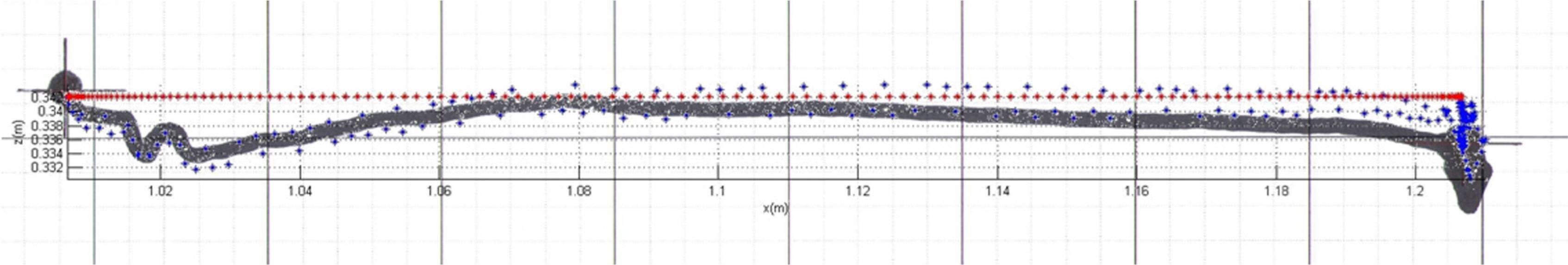
Fig. 23 illustrates a graph showing the position of the object from the underwater robot and the trajectory of the end-effector. The red dots denote the positions of the target object from the underwater robot, and the blue dots are the positions of the end-effector calculated based on the joint angle fed back from the manipulator. As in the previous experiments, the end-effector first approaches the position of the target object, and after the target object and the end-effector move sufficiently close, we can see that the end-effector continuously tracks the target object as it moves. In the graph, it can be seen that the red dots are constantly moving owing to the navigation errors, which are the position control errors of the underwater robot due to the effect of the movement of the manipulator. It can be noted that the end-effector continuously tracks the change in the relative distance of the target object in underwater environment. Here, the graph in Fig. 23 presents the data in the state when the end-effector is sufficiently close to the target object, which is 10 s after the case in Fig. 14.
End-effector trajectory for an underwater movement obtained from the experiment
Line drawing scenes using a pen held by end-effector
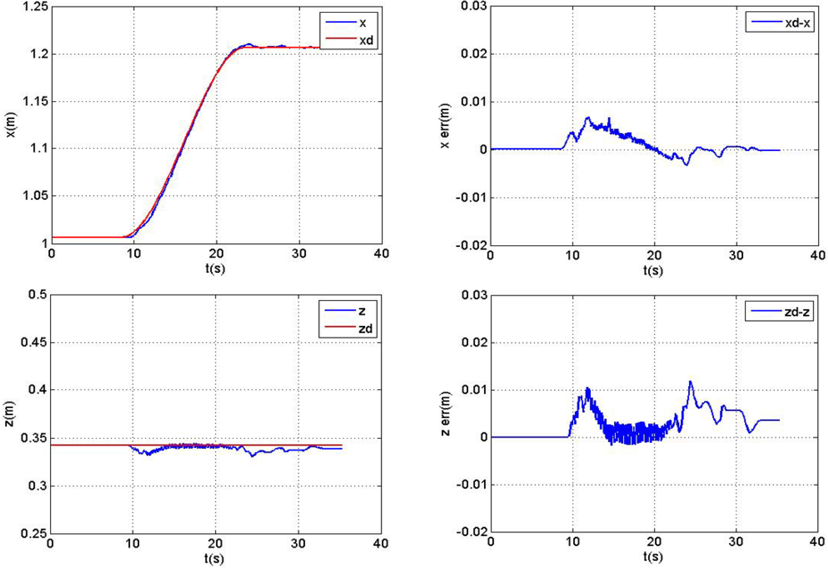
Fig. 24 depicts a graph of the end-effector position and the position error with the target object in underwater environment. In the initial stage of the tracking, we can observed that the end-effector moves toward the target object. During the end-effector tracking of the subject, an overshoot of approximately 20 mm occurs at approximately 17 s. Subsequently, it can be observed that the end-effector tracks stably according to the movement of the target object after approximately 20 s. At this time, an error of approximately 4 mm occurs in the X direction and of approximately 2 mm each occurs in the Y and Z directions. It can be confirmed that unlike the previous experiments on the ground, the effect of the control performance deterioration of the actuator by gravity is reduced.
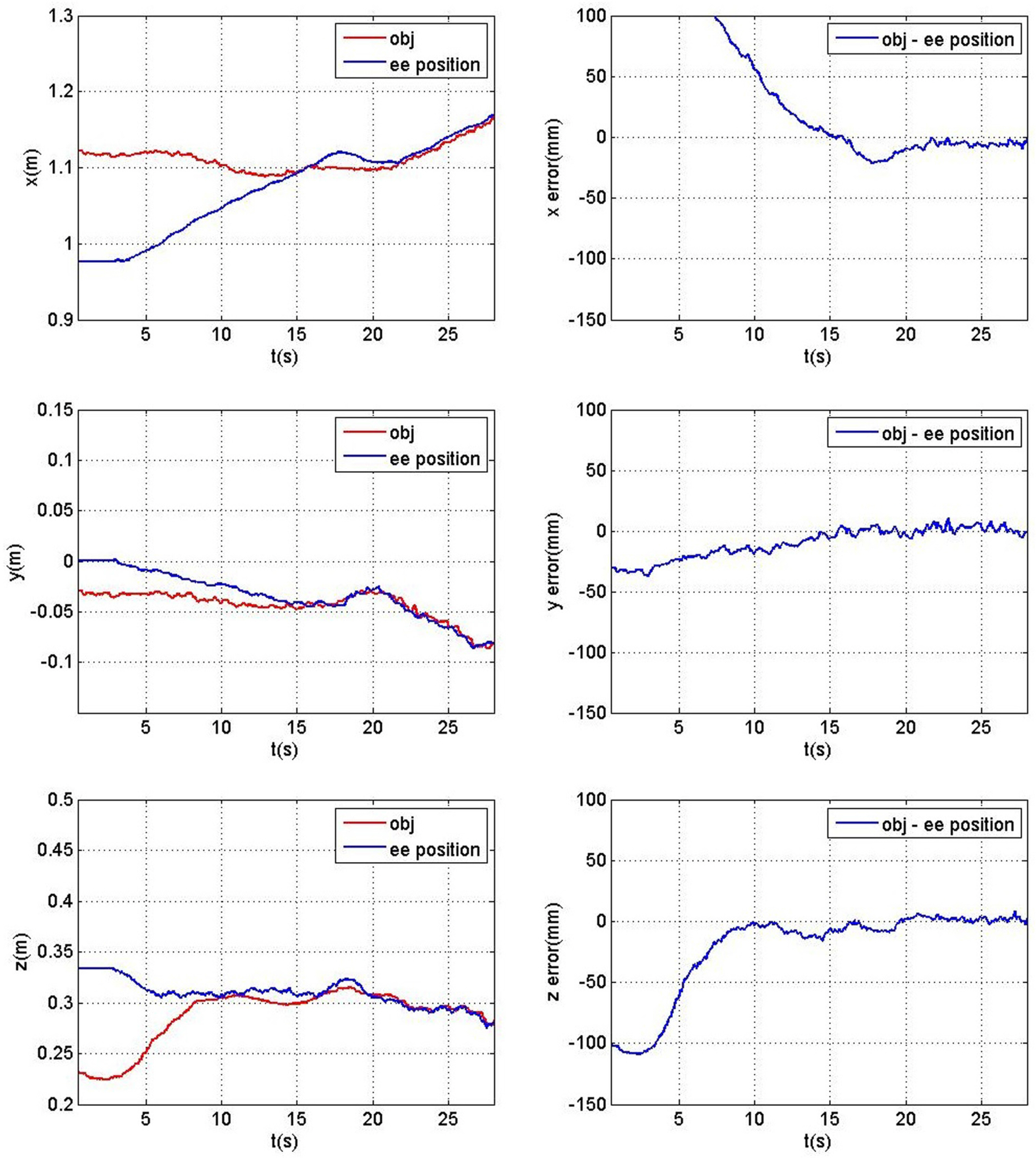
Position and error for an underwater movement obtained from the experiment
5. Conclusion
In this study, the tracking performance of an ECA ARM 7E Mini model manipulator installed on an underwater robot for autonomous manipulation was verified. For the kinematic description of the manipulator, a prismatic joint output was converted into a revolute joint output, and velocity control was performed based on closed-loop inverse kinematics. To respond to the changes in the position of the underwater robot due to disturbances, a manipulator control was implemented to track a target object. However, since rapid tracking of the manipulator adversely affects the position control performance of the underwater robot, it was ensured that the end-effector tracks the target object without exceeding the specified velocity. The performance of the tracking algorithm was verified by performing a simulation tracking a linear trajectory and a moving target object using the Gazebo simulator. The performance was further demonstrated using an actual manipulator and conducting an experiment the identical to the simulation. Based on the tracking performance verification on the ground, the manipulator was installed on an underwater robot, to examine the underwater tracking performance. From the results of the experiment on the ground, it was confirmed that compared to the simulation result, an error was caused by the poor tracking performance of the end-effector, resulting from a lack of the control performance of the joint actuator under low velocity and load conditions. However, the results of an underwater experiment demonstrated that the tracking performance degradation of the actuator was reduced. A planned follow-up of this study is as follows. We aim to perform autonomous underwater manipulation by the manipulator by improving the tracking error of the target tracking algorithm of the manipulator used in this study. We aim to apply the results to autonomous decision-making for the movement of a manipulator in a work space and the movement of an underwater robot and the manipulator when the manipulator installed on the former interacts with a target object. Furthermore, to reduce the position error of the manipulator, we aim to apply dynamics-based control, such as a mass matrix
Acknowledgements
This study was conducted under the projects of “Development of 3D object recognition and robot-robot arm motion compensation control generic technology for autonomous underwater manipulation” and “Development of core technology on the cyber physical system of underwater robot (CPOS),” which were conducted as the institutional projects of KRISO.