Analysis of Effect on Seawater Flow Change and Circulation Inside Port Due to the Construction of South Breakwater and Weir at Gamcheon Port
Article information

Abstract
In this study, numerical simulations are used to analyze the effect of the south breakwater and weir on seawater flow change and circulation within the Gamcheon port. Flow patterns in the eastern direction are particularly affected by the breakwater during the ebb tide and current velocity is slightly reduced by construction of the weir. Additionally, seawater circulation is reduced by both features. In order to increase seawater circulation, a seawater flux structure is needed on the west breakwater. A weir-type structure will be more efficient than a seawater flux culvert.
1. Introduction
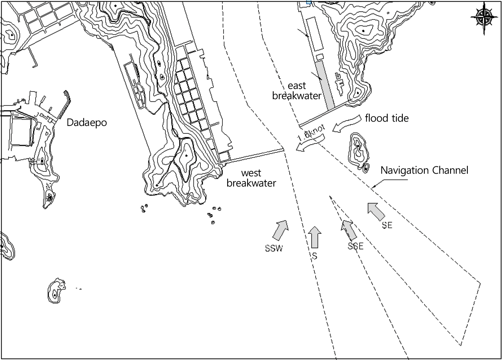
Gamcheon Port is located on the eastern side of the southern coast of Korea. Although it is a harbor that supports the Busan Northern Port, it opens to the south, which is its main wave direction. Normally, there is a high appearance ratio of waves with heights exceeding 0.5 m, which is the critical depth for loading medium and large ships. During typhoons, there are many regions in the port where the wave height exceeds 3.0 m. The outer parts of the port open directly to the deep sea, without any natural sheltering topography such as islands. Because the water around Gamcheon Port is deep and the sea bed is mild slope, deep-water waves enter the port entrance without being reduced. In recent years, the cargo volume of the port has increased, as has the number and size of ships that use the port. As such, plans have been examined for rearranging or remodeling the port’s existing outer facilities, in order to increase ship navigation safety. Remodeling the port’s facilities could also increase harbor tranquility along the outer side of the Gamcheon Port fish market and improve the usage efficiency of the harbor’s facilities. Currently, the Gamcheon Port is not sufficiently protected from waves travelling from the south, and specially, Busan Metropolitan city is promoting the construction of a public fish market behind the east breakwater which affects harbor tranquility. The Ministry of Planning and Budget has conducted a feasibility study on maintenance projects for Busan’s Gamcheon Port. It was found that the construction of another breakwater was not economically feasible (B/C(Benefit/Cost): 0.46), but it is necessary to look for alternatives through numerical analysis, hydraulic model experiments, ship handling simulations, etc. Outer facilities, such as the southern breakwater, were constructed to improve the tranquility of Gamcheon Port, in order to revitalize it and boost its level of usage. However, the tidal currents between Dudo Island and Danggangmal are strong, and ship navigation can be hazardous in this area. Accidents have occurred in which ships entering Gamcheon Port have struck the west breakwater (Fig. 1). Because the construction of a south breakwater was expected to exacerbate this phenomenon, a current-reduction facility (weir) was installed between Dudo Island and Danggangmal to mitigate the current.
Area for this study
Before the construction of the south breakwater, seawater circulation in Gamcheon Port was facilitated by inflow between the east and west breakwaters, from the combined action of open-sea waves and tidal currents between Dudo Island and Danggangmal (Fig. 1). However, the construction of the south breakwater weakened the open-sea waves entering the port and the current between Dudo Island and Danggangmal was reduced by the installation of the weir. This unavoidably changed the seawater flow in the port and affected circulation. The installation of a seawater flux structure such as culvert was planned on the existing west breakwater. However, due to concern regarding reduced seawater circulation in the port, it is necessary to review the planned location of this structure. An example of a seawater flux structure installation is the seawater exchange breakwater that was installed in Jumunjin Port, on the east coast of Korea, to improve seawater circulation in the port. Simulations (Oh et al., 2002) were performed to confirm its effectiveness, and it was completed in 2004. It successfully alleviated pollution in Jumoonjin Port by promoting seawater circulation within the port. In addition, studies have examined the effects of seawater flux structures on the circulation of seawater in ports (Kim et al., 2003; Kim and Kim, 2003; Jang et al., 2010). Recently, Hong (2016) examined how seawater circulation is affected by loading and unloading at the pier bridge of the New Busan Port.
The goal of this study is to use a numerical simulation to analyze changes in the port’s flow field due to the construction of the south breakwater and weir and to evaluate the efficiency of the seawater circulation flux structure. In the flow model, the weir is seen as a porous plate and depicted using a quadratic loss term. The loss coefficient was applied according to the penetration rate, by calculating the amount of flow penetrating the weir. In addition, the seawater flux structure was regarded as a culvert and various positions along the breakwater were analyzed. Due to the difference in water levels before and after the culvert, 6 different types of flow regimes were classified, and the amount of flow penetrating the submerged culvert was then calculated.
2. Mathematical and Numerical Models
To analyze the port seawater flow, this study used the seawater flow model developed by Hong (2009) and Hong (2012). This model was partially modified for the seawater circulation analysis in order to examine the effects of the weir and the seawater flux structure on the flow field.
2.1 Outline of Mathematical and Numerical Seawater Flow Model
This study used a 3D model that was developed by Hong (2012). The model was verified by comparing its simulation results with field observations (Hong, 2012). The mathematical model uses a σ coordinate system, and its depth-averaged continuous equation in the σ coordinate system is Eq. (1), while the equations for the amount of flow in the horizontal direction ξ and the η direction are Eqs. (2) and (3), respectively.
Here, Jξξ and Jηη are the Jacobian values in the horizontal coordinate system (ξ, η). U and V are the depth-averaged flow rates in the horizontal direction. Q is the inflow and water yield per unit area.
Here, f is the Coriolis constrant. Sξ and Sη are the flow source and sink in the ξ and η directions, respectively. u and v are the flow in the horizontal ξ, direction and the η direction, respectively. w̄ is the the relative flow in regards to the vertical ζ direction’s movement σ plane. It is calculated from the continuous Eq. (1).
The numerical model uses a staggered grid system and the 3D governing equation is finite-difference discretized, in relation to time and space. In the vertical direction, it used a σ coordinate grid with the same number of layers for all areas in the horizontal direction, irrespective of changes in water depth.
The ADI (alternating direction integration) scheme (Leendertse and Gritton, 1971; Leendertse et al., 1973) was used as a basic method for integrating time historical data. A method that improves upon the ADI scheme (Stelling and Leendertse, 1991) was used to perform spatial discretization of the horizontal nonlinear term. The horizontal flows between the vertical layers were coupled with each other due to the vertical nonlinear term and the viscosity term, and fully implicit time integration was performed on the mutually connected vertical terms to remove the instability of solution. Spatial separation was performed by using second-order central differencing on the nonlinear term and first-order central differencing on the viscosity term.
2.2 Weir Modeling
If there are obstacles such as weirs in a flow field, a difference in water levels occurs upstream and downstream from the obstacle. Because of this, a pressure gradient occurs at the location where the weir is installed. However, in flow models, there may be problems with the solution accuracy, even if the grid intervals are minimized to depict presure gradient on the grid numerically. Therefore, this study considered the weir to be a porous plate and performed parameterization to depict the energy loss caused by the structure at the grid boundaries. That is, energy loss was depicted by adding the quadratic loss term in Eqs. (4) and (5) to the source term in the momentum equations, Eqs. (2) and (3) (Hong et al., 2008).
Here, closs − u and closs − v are the energy loss coefficients. Eqs. (4) and (5) show the energy loss caused by the reduced cross section. The subcritical flow caused by the reduced cross section is related to the difference in water levels on either side of the hydraulic structure, and is shown in Eq. (6).
Here, μ(0 ≤ μ ≤ 1)is the cross section reduction coefficient. A is the wet area. ζu and ζd are the water levels upstream and downstream of the weir, respectively. Both sides of Eq. (6) are squared and divided by 2μ2A2Δx to create Eq. (7). Making the right side of Eq. (7) equal to Eq. (4) results in Eq. (8).
The relational equation in Eq. (9) can be found by comparing the second and third terms in Eq. (8). If the contraction coefficient is known from this relational equation, the energy loss coefficient can be determined.
However, it is not easy to calculate the contraction coefficient for a porous plate, unlike a regular plate that blocks the front of the flow. For this study we selected a method that calculates the contraction coefficient directly from the results of tank experiments, using the relationship between the first and third terms in Eq. (8).
2.3 Seawater Flux Structure Modeling
The seawater flux structure was regarded as a culvert, and the flow passing through it can be calculated using Eq. (10) due to the difference between the water levels upstream and downstream of the culvert.
Here, μ is the culvert loss coefficient (dimensionless). A is the area of the culvert opening (in m2). ζintake and ζculvert are the water levels at the intake and outlet, respectively.
The flow can penetrate only part of the culvert’s cross section due to its installation location, slope, etc., and several flow regimes can occur in the culvert. Eqs. (11) and (12) define the water levels upstream and downstream from the culvert. Eqs. (14) to (19) depict the classification of 6 types of flow regimes within the culvert according to the water level limit defined in Eq. (13) (Jagers and van Schijndel, 2000).
Here, Hc is the critical depth and ζculvert is the culvert’s vertical location. ζups and ζdowns are the culvert’s upstream and downstream tide levels, while W is the culvert’s width. In Eqs. (14) and (19), H* is the modified depth, and L is the length of the culvert. n is Manning’s coefficient (in m1/3/s). cD1/2/33 is the discharge coefficient and α is the energy loss correction coefficient.
Type 1 (Supercritical flow with critical depth at intake; steep culvert slope)
Type 2 (Supercritical flow with critical depth at outfall; mild culvert slope)
Type 3 (Tranquil flow)
Type 4 (Submerged flow)
Type 5 (Rapid flow at inlet)
Type 6 (Full flow free at outlet)
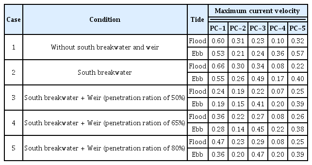
The amount of flow is calculated according to the flow classification in Eqs. (14) to (19), and the flow regime classifications are shown in Table 1. As shown in Table 1, the flow regimes are classified according to the range of water levels upstream and downstream of the culvert.
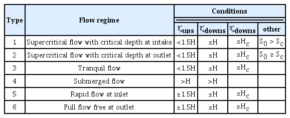
Flow regime due to water level differences on either side of the culvert
3. Establishing the Numerical Model
3.1 Establishing the Seawater Flow Model
As shown in Fig. 2, a variable grid system was used as the wide area grid for the seawater flow numerical model experiments. The grid interval was variable, and had a default value of 250 m with a dx of 200–500 m and a dy of 300–600 m. For open boundary conditions of the target sea area, Matsumoto et al. (2005) created a simulation using TOPEX Poseidon satellite depth data and used the results to construct a partial tide table, from which 16 partial tide values (2N2, J1, K1, K2, L2, M1, M2, MU2, N2, NU2, OO1, O1, P1, Q1, S2, T2) were selected for this model. For the eddy viscosity, 10m2/s was used uniformly across the entire wide area. For the floor frictional force, 45m1/2/s was used for the entire sea area, based on the Chezy equation. The wind data in this study was sourced from observational data recorded in Busan Port between 2016 and 2018, and was applied uniformly to the entire sea during whole time. The friction coefficient between the wind and sea surface was set as 0.0026. To verify and certify the established wide area model, the observed tide level and flow rate field, from points P1 to P4 in Fig. 3, were compared with the calculated values from the seawater flow numerical experiments performed in this study, as shown in Fig. 4.

Coarse grid system
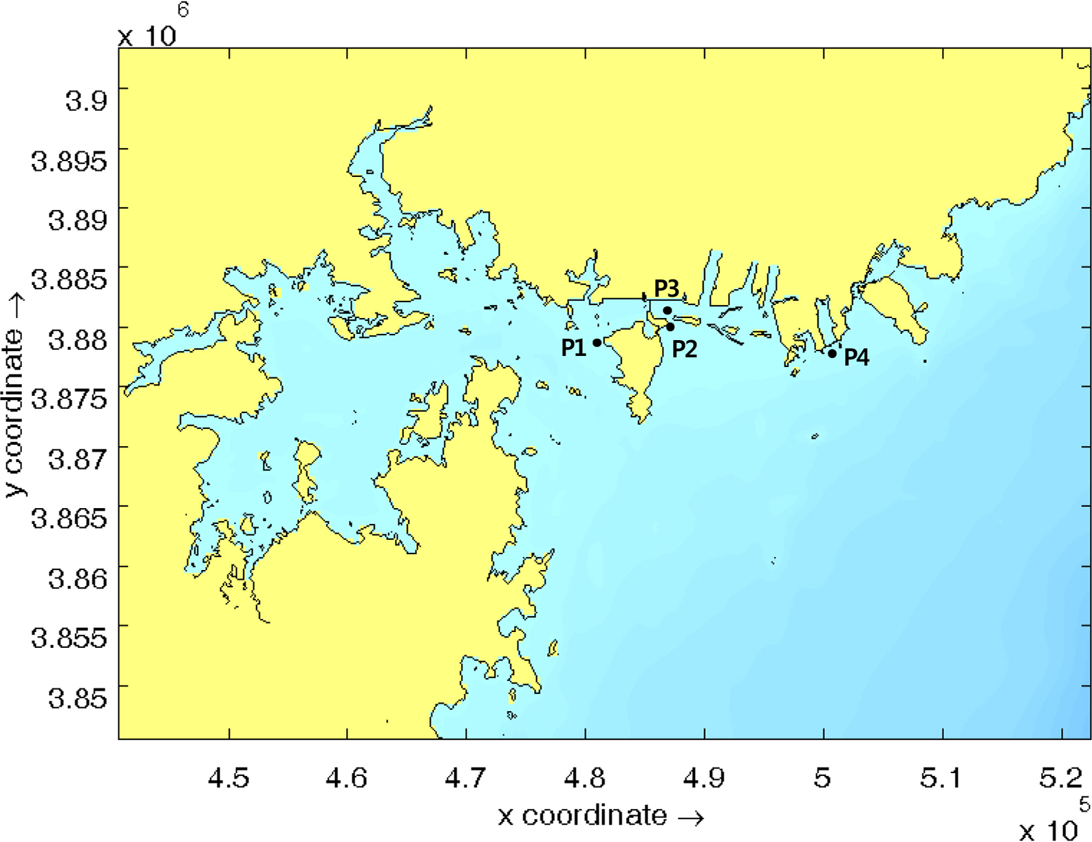
Position for model verification

Model calibration through comparisons between measured results (dotted line) and simulation results (solid line)
From the regional results, the boundary conditions of the specific areas were transferred as shown in Fig. 5, and seawater flow simulations were performed on specific areas. The specific area grid system that was selected for the seawater flow numerical model experiments was a variable grid system with a dx grid interval of 20–100 m and a dy of 15–100 m, as shown in Fig. 6. The eddy viscosity of the entire area was set as 5 m2/s. The floor frictional force was set as 30 m1/2/s for the entire sea area, based on the Chezy equation. The same observational wind data, from 2016–2018 in Busan Port, was again applied uniformly to the entire sea area over time. The friction coefficient between the wind and the sea surface was set as 0.0026.
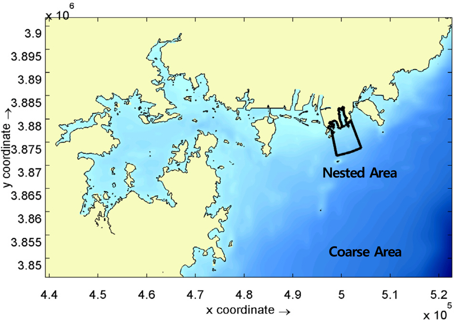
Coarse and Nested grid
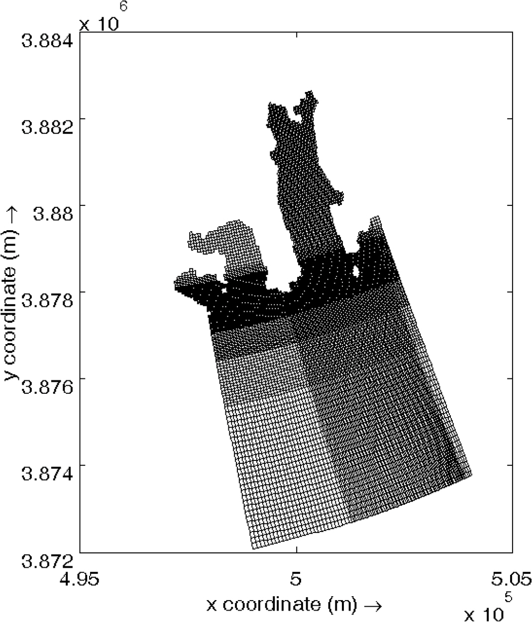
Nested grid system
3.2 Calculating the Weir Loss Coefficient
When the quadratic loss term in Eqs. (4) and (5) is used to depict submerged structures in the flow model, the most important element is a rational calculation of the loss coefficient, closs. This study calculated the amount of flow that penetrated the weir (illustrated in Fig. 7) and applied the loss coefficient that resulted from the penetration ratio. For example, when the target penetration ratio was 50%, the numerical model experiments were performed by changing the loss coefficient until the amount of penetrating flow over the course of 14 days was 50% of the flow before and after the installation of the weir. Fig. 8 shows the change in flow before and after weir installation. The loss coefficients, calculated via the method above, were 2.1, 1.1, and 0.58 when the weir penetration ratios were 50%, 65%, and 80%, respectively.
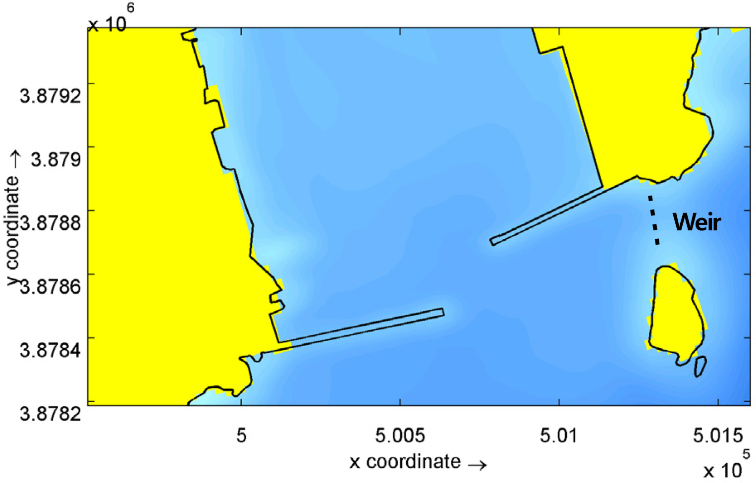
Position of weir

Change of discharge according to construction of weir
3.3 Calculating the Seawater Flux Flow of culvert due to Waves and Applying It to the Flow Mode
When the culvert was added to the model to simulate the installation of a seawater flux structure at the east breakwater, the difference in water level on either side of the culvert were mainly due to waves, rather than tides, and this created flow in the seawater flux structure. However, when a numerical model experiment is performed for a long period, as is the case with the seawater flow model, it is inefficient to use an integral time applied to short periods such as waves. Therefore, we calculated the 6 types of culvert flow regimes from the tide model, by using the mean wave height of the integral period for the sea-facing side of the breakwater, and the tide level height for the port-facing side. The amount of penetrating flow was then calculated, and these values were used as the source and sink in the seawater flow numerical model experiments (Fig. 8).
4. Results Analysis
4.1 Changes in Seawater Flow Around the Breakwater due to the South Breakwater and Weir
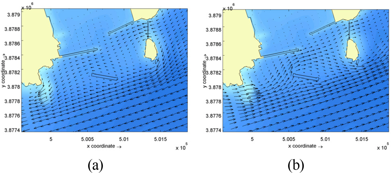
Numerical model experiments were conducted on the 5 scenarios shown in Table 2 in order to examine how the flow field of the surrounding ocean area was affected by the construction of the south breakwater and the weir between Dudo Island and the east breakwater. Figs. 9 to 13 show the flow fields for each experiment case, during ebb and flood tides. In Case 2, in which only the south breakwater had been built, it can be seen that during flood tide, the flow direction at sea area between main ground and Dudo was not very different to the tangential direction of the south breakwater, and the south breakwater did not have a large effect, compared to the scenario before its construction. However, during the ebb tide, the eastward flow was affected by the south breakwater. Also, in the cases where the weir was constructed (Case 3, Case 4, Case 5), the overall flow was not changed, but the weir reduced the flow rate on either side of it. The weir affected the port entrance area slightly. This effect increased marginally when the penetration ratio was increased from 50% to 65%, and to 80%.
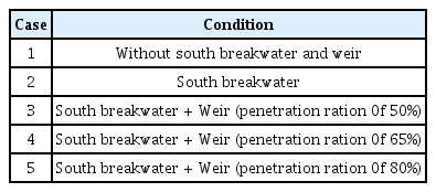
Numerical model scenarios for the investigation of the effects of south breakwater and weir on flow

Flow velocity field for Case 1 during (a) ebb tide and (b) flood tide
Flow velocity field for Case 2 during (a) ebb tide and (b) flood tide

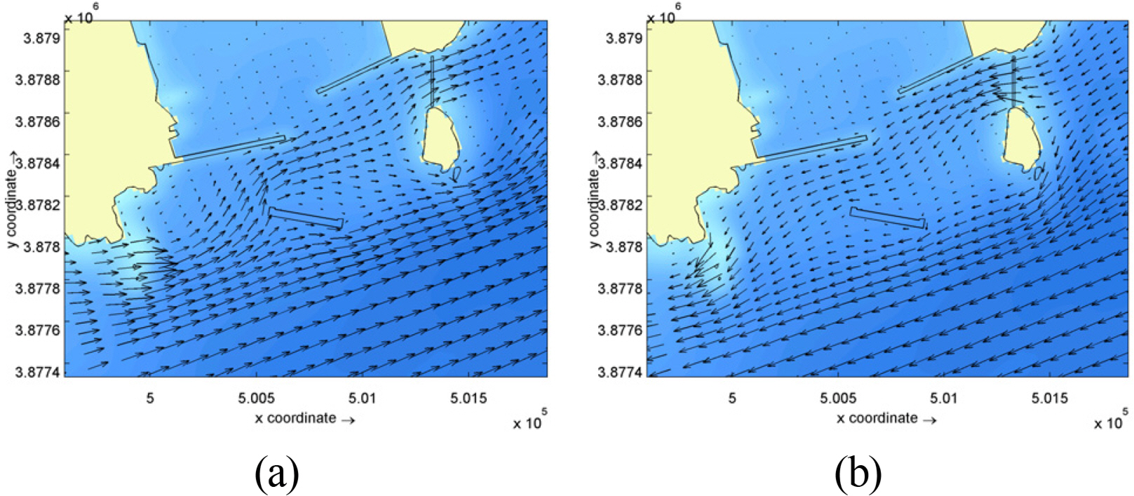
Flow velocity field for Case 3 during (a) ebb tide and (b) flood tide
Flow velocity field for Case 4 during (a) ebb tide and (b) flood tide

Flow velocity field for Case 5 during (a) ebb tide and (b) flood tide
As mentioned before, the flow rate at the Gamcheon Port entrance waterway increased as a result of the construction of the south breakwater, and this affected ships entering and exiting the harbor. Therefore, in order to control the flow rate around the port entrance, a weir was installed at the north end of Dudo Island, and its construction is linked to a change in flow rate around the port entrance. The flow rate around the south breakwater was quantified and examined at the locations in Fig. 14. The strongest flow rates at each point are shown in Table 3. At PC1 (the front of the west breakwater) the flow was greater in Case 2 than in Case 1, due to the construction of the south breakwater. However, as seen in Cases 3, 4, and 5, the flow rate decreased after the weir was installed. In the case with a low penetration ratio (Case 3), it decreased further. At point PC2 (port entrance), a phase difference occurred due to the combined effect of the south breakwater and the weir, and no clear increase or decrease occurred. The flow rate was less than 0.3 m/s. However, at point PC3 (the front of the east breakwater), the strongest flow rate increased to 0.49 m/sec due to the effect of the south breakwater. At points PC4 (between Dudo Island and the south breakwater) and PC5 (the front of the south breakwater), the flow decreased in comparison to Case 1, due to the shadow effect of the south breakwater. The amount of decrease was determined by the south breakwater rather than the effect of the weir.
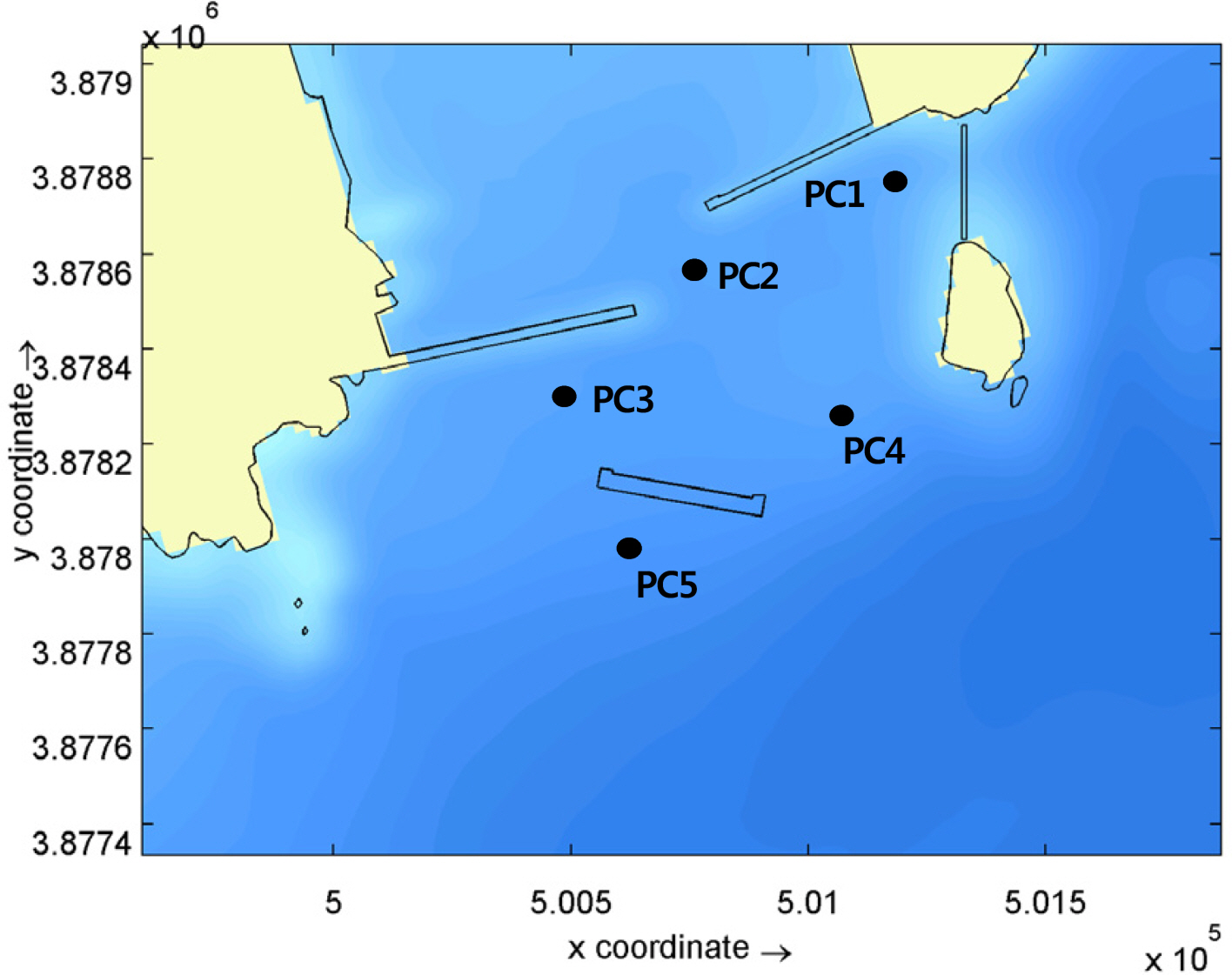
Designated positions of calculating current velocity
The flow rate distribution during the strongest ebb tide is shown in Fig. 15. Compared to Case 1, Case 2 showed flow rate changes around the south breakwater, and Cases 3, 4 and 5 show changes in the flow field around the weir. Also, it was found that the trends were very similar to those of the flood tides. That is, during flood tide, the flow direction at northern sea area of Dudo was not very different from the tangential direction of the south breakwater, and the effect of the south breakwater was not large. However, during ebb tide, the eastward flow was affected by the south breakwater. In addition, when the weir was constructed, the overall flow was not changed, but the weir reduced the flow rate on either side of it. The weir affected the port entrance area slightly. This phenomenon tended to occur slightly more when the penetration ratio was increased from 50% to 65% and 80%.

Maximum ebb current velocity
4.2 Effect of Construction of the South Breakwater and Weir Construction on Port Seawater Circulation
This study examined the changes in flow rate at the port entrance due to the construction of the south breakwater and weir, and the resulting effects on port seawater circulation. The effects of culvert to be installed at the west breakwater were also examined. To examine seawater circulation, this study performed a drogue drop experiment (Fig. 16(a)), which is a particle tracking method. 128 drogues were dropped into the port and one month later their positions and the number of drogues remaining in the port were noted, to estimate the transport patterns of materials that are dropped in the port. In order to conduct detailed quantitative port seawater exchange experiments while considering the circulation patterns obtained from the drogue drop experiment, we used a COD (Chemical oxygen demand) diffusion simulation, which only considers the physical dispersal process. To calculate the seawater exchange rate, the initial COD concentration in the Gamcheon Port was set at 100 ppm, and the changes in concentration after one month were measured at 27 major points in the port, as shown in Fig. 16(b). The model developed by Hong (2010a) and Hong (2010b) was used in the COD concentration diffusion simulation.

Numerical experiment for the investigation of seawater circulation in port (a) Drogue drop experiment (+: initial drogue position), (b) position for the investigation of COD concentration
Fig. 17 shows the simulated drogue locations after 1 month for the cases shown in Table 4. Due to the construction of the breakwater, the amount of inflow into the port was reduced. In Case 2, a larger number of drogues remained in the port, and they were distributed over a larger area, while the seawater circulation was lower than in Case 1. When seawater flux structures were installed at the center part of the west breakwater (Case 3) and the head of the breakwater (Case 4) to improve seawater circulation, the number of drogues was the same as in Case 2, but the distribution area was slightly different.
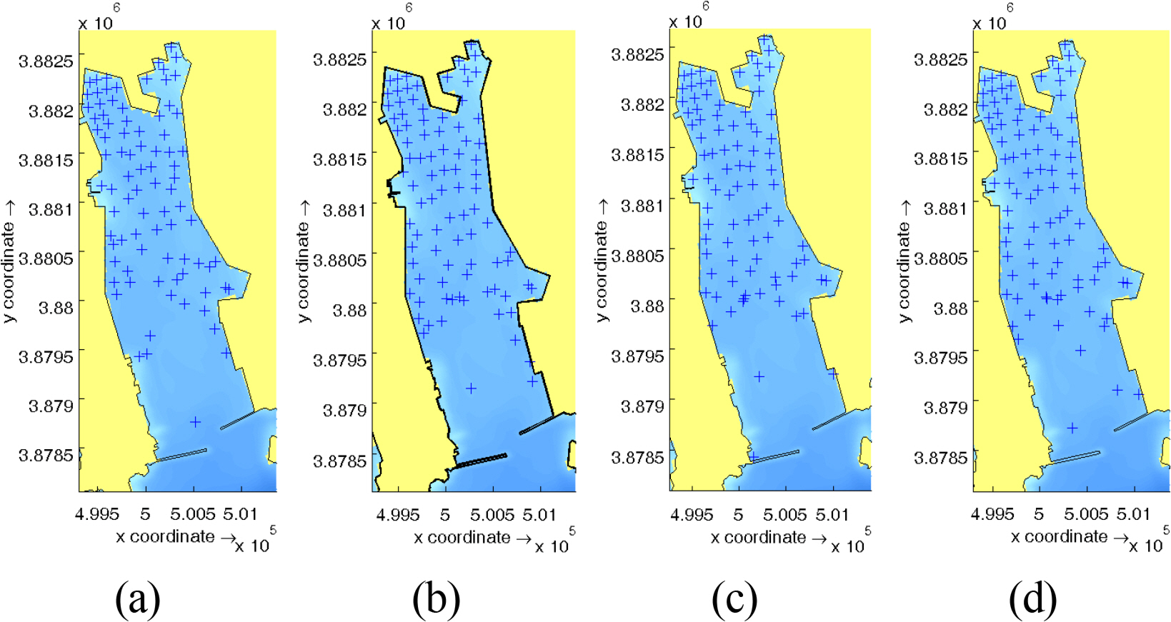
Drogue positions 1 month into simulation

Numerical experimental cases for the investigation of seawater change
This shows that seawater flux structures are somewhat effective in improving seawater circulation. As such, there is a need to quantitatively examine these seawater circulation improvements. To do this, COD concentration changes were examined, as mentioned previously.
The initial COD concentration in Gamcheon Port was set at 100 ppm, and the concentration changes at major points in the port were examined after 1 month simulation, to examine how seawater circulation is affected by factors such as the south breakwater, the location of the seawater flux structure, the scale of the seawater flux structure, the weir penetration ratio, and the weir overflow amount. Fig. 18 shows the concentration distribution after one month in the scenario with the south breakwater and weir (penetration ratio of 50%), before and after construction. It was found that the overall COD concentration in the port increased due to the construction of the south breakwater and the weir.
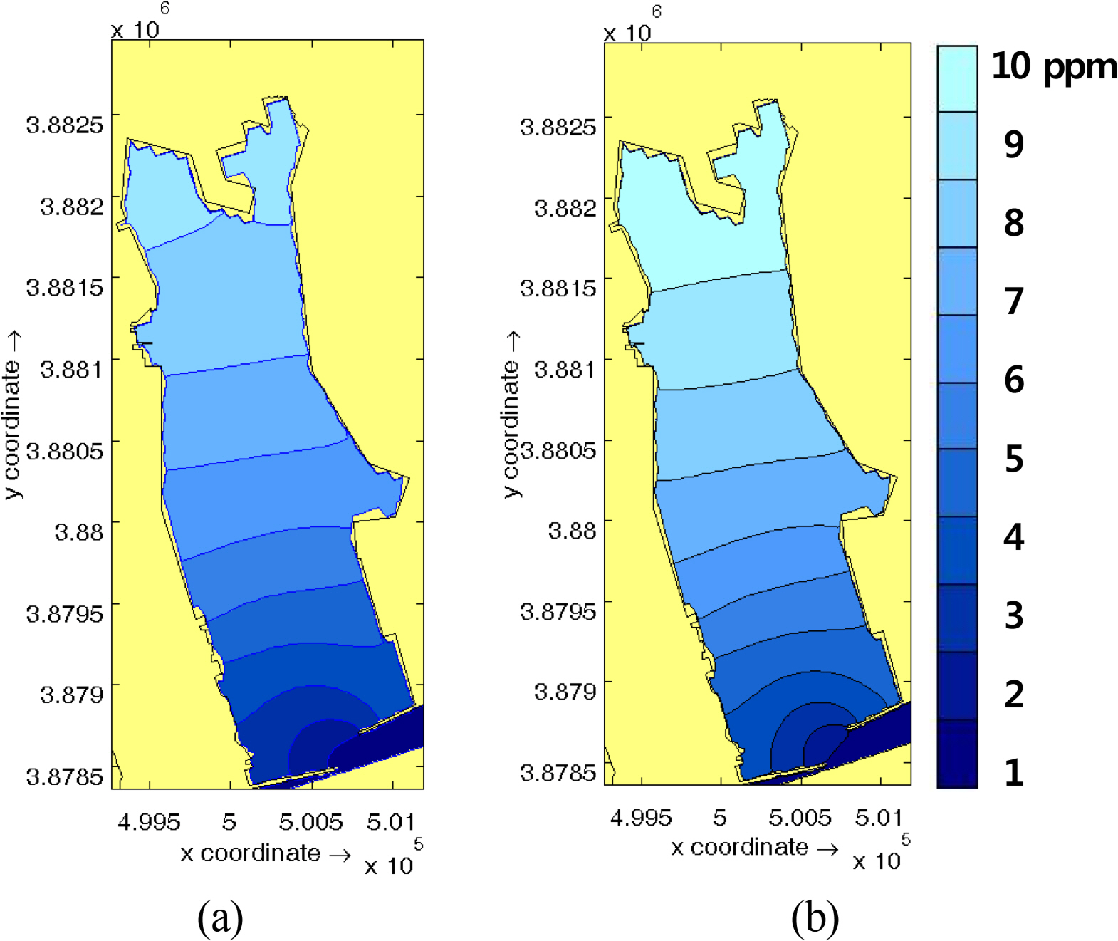
Change in COD concentration after 1 month of COD simulation (a) before construction of south breakwater and weir, and (b) after construction of south breakwater and weir, with 50% penetration ratio
To provide a quantitative examination, Table 5 shows the concentration changes at the examination points in Fig. 16(b) after one month, with and without the breakwater and weir construction. The final column of Table 5 depicts the change in concentration between these scenarios as a percentage [= 100 × (concentration after installation – concentration before installation) / concentration before installation]. The concentration increase ratios show that closer to the west breakwater, the increases in concentration tend to be larger. This means that the construction of the south breakwater and weir caused the overall seawater circulation pattern at the port entrance to flow in a clockwise direction.

Change of COD concentration after 1 month of COD simulation
As mentioned above, the seawater circulation pattern in the port changed to a clockwise direction due to the construction of the south breakwater. The seawater flux structure should therefore be installed on the west breakwater. It is necessary to examine how the change in COD concentration, before and after construction, varies according to the different locations and scales of the seawater flux structure. Fig. 19 shows the different positions of the seawater flux structure (west, east, center). The scale was increased to 130% and 150% when the structure was located in the center of the west breakwater. Fig. 20 shows the concentration increase ratios obtained from major points in the simulation, with the seawater flux structure at different locations. In terms of seawater circulation in the port, it is most advantageous to install the seawater flux structure on the western end of the west breakwater. Fig. 21 shows the variation in concentration increase ratios, obtained from major points in the simulation, according to increases in the cross-sectional area of the seawater flux structure. As the area increased, the change in COD concentration decreased, and the seawater circulation in the port improved. However, with the exception of some points, the decrease was slight, and the degree of improvement was not large.
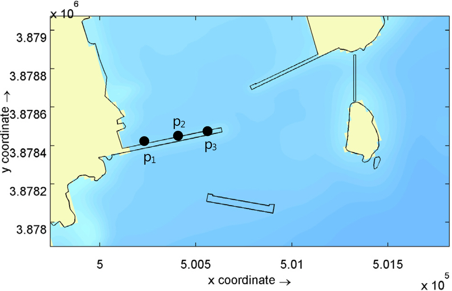
Position of seawater flux structure (p1: West, p2: Center, p3: East)
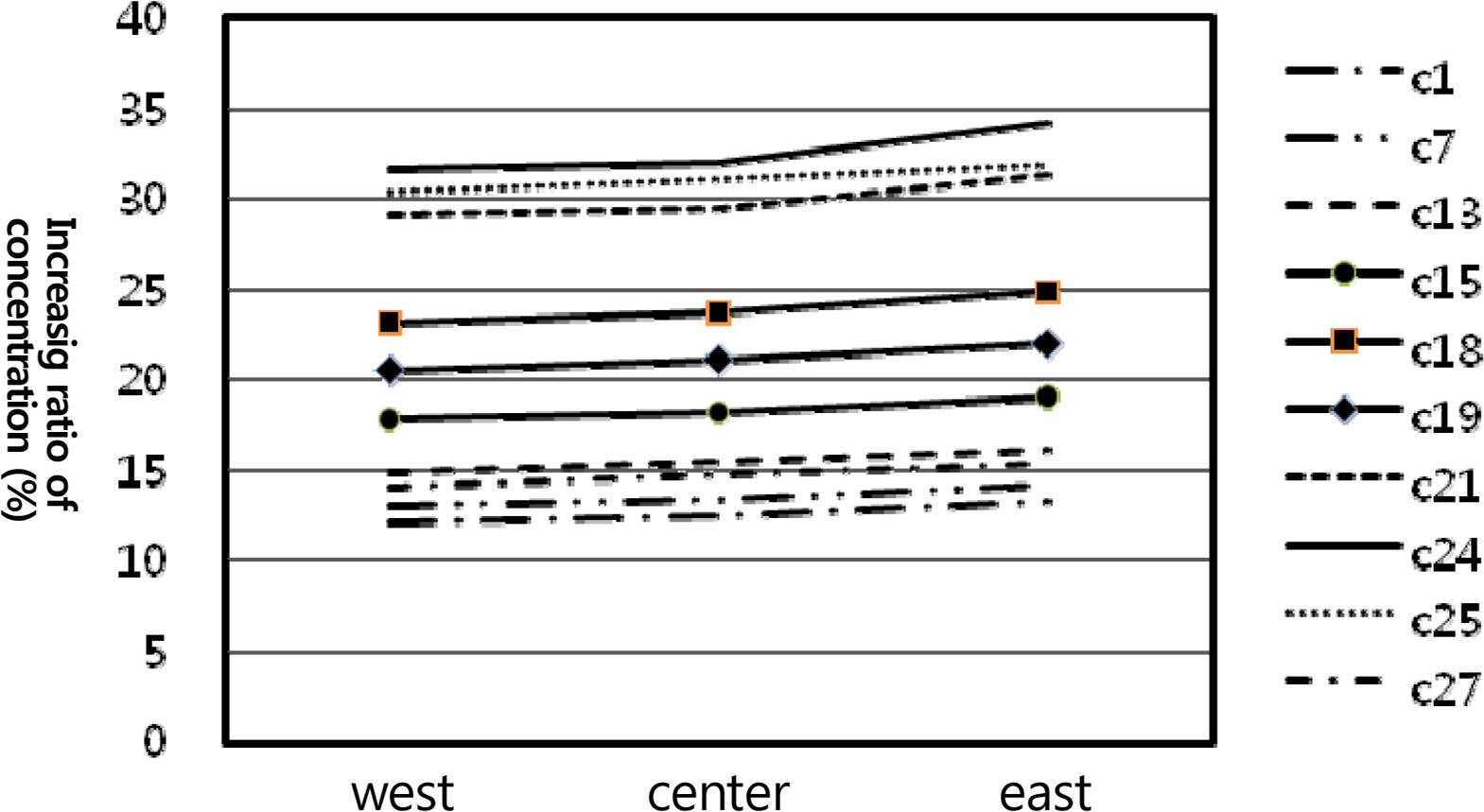
Variation of concentration increase ratio with position of seawater flux structure
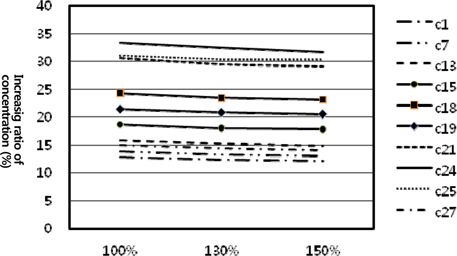
Variation of concentration increase ratio with size of seawater flux structure
Fig. 22 shows the variation in the concentration increase ratio due to changes in the weir penetration ratio. As the penetration ratio increased, the concentration increase ratio rapidly decreased, and the seawater circulation in the port was effectively improved. It is believed that this occurred because the westward flow rate increased during the flood tide, and inflow through the port entrance increased as the weir’s penetration ratio increased.
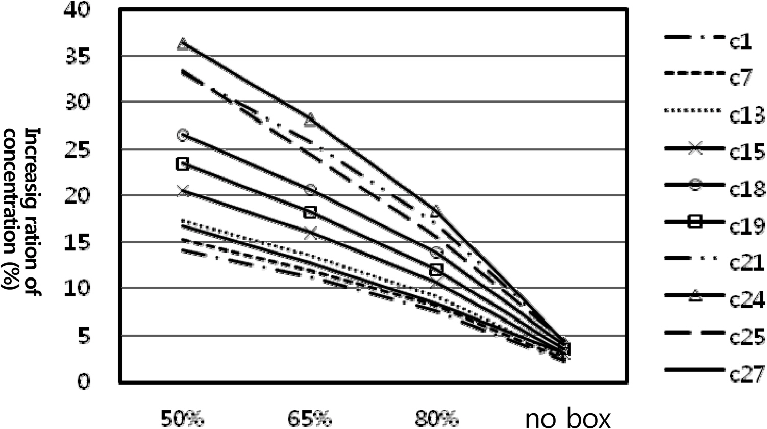
Variation in concentration increase ratio due to changes in penetration ratio of seawater flux structure
The seawater flux structure that was installed to improve seawater circulation in the port depends on open sea waves because it operates based on the upstream/downstream difference in water levels that is mainly caused by waves. In contrast, a weir can continuously provide flow to the port because the flow that is accumulated within the structure due to waves is released into the port. Therefore, this study calculated the percentage change in COD concentration within the port after construction of the south breakwater and weir, while altering the amount of flow provided by the weir to the port. The flow that was supplied to the port was treated as the flow source. The weir was located on the western end of the west breakwater, based on the improvement created by the seawater flux structure being placed there. Fig. 23 shows the variation in concentration increase ratio due to the amount of flow provided by the weir. As the flow provided by the weir increased, there was a greater improvement in the seawater circulation in the port.
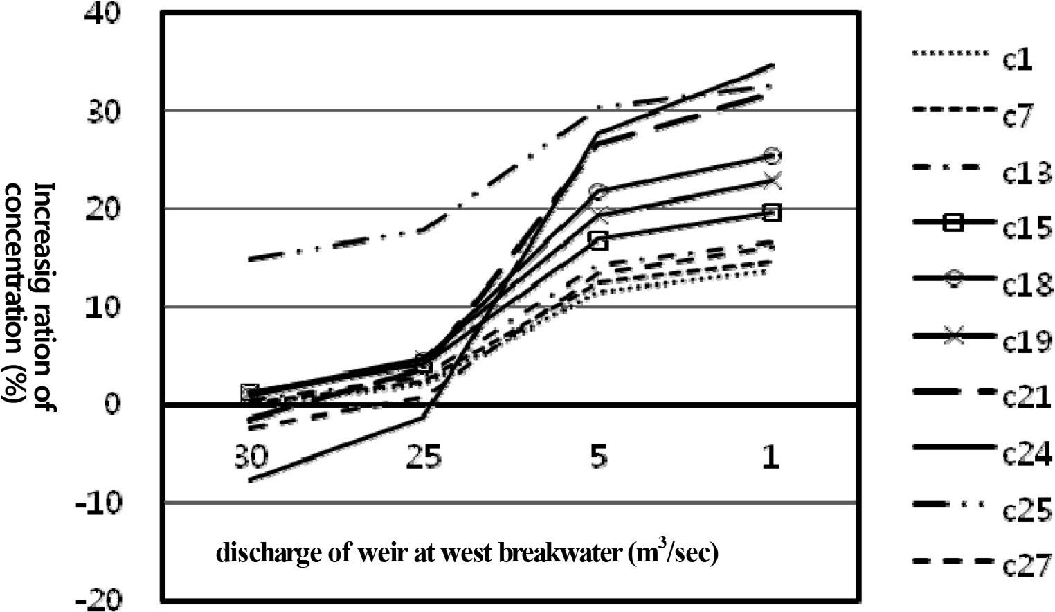
Variation in concentration increase ratio due to increasing discharge of at west breakwater
The results above show that the most efficient method for improving circulation of the Gamcheon port seawater is to increase the weir’s penetration ratio as much as possible. Increasing the cross-sectional area of the seawater flux structure did not cause a large improvement in seawater circulation. However, when the amount of flow provided by the weir was increased, there was a clear improvement in seawater circulation. Therefore, it is beneficial to use an weir at the west side of the west breakwater, while properly controlling the amount of provided flow, rather than using a seawater flux structure. Increasing the weir’s penetration ratio as much as possible, in limited circumstances, is beneficial for improving seawater circulation in the port.
5. Conclusions
This study analyzed the nearby sea flow changes caused by the construction of the south breakwater and weir at Gamcheon Port. The results showed that when the south breakwater was constructed, the flow direction from Dudo Saigol during a flood tide was not very different from the tangential direction of the south breakwater, and the effect of the south breakwater was not large. However, during ebb tide, the eastward flow was affected by the south breakwater. In addition, when the weir was constructed, the overall flow was not changed, but the flow rate on either side of the weir was reduced. The weir affected the port entrance area only slightly, but the effect was slightly greater when the penetration ratio was increased from 50%, to 65%, and to 80%.
In addition, this study examined the effects of the south breakwater and weir construction on port seawater circulation caused by changes in the flow rate at the port entrance. The results show that there is a need to install a seawater flux structure to prevent pollution problems occurring due to reduced seawater circulation in the port. The most efficient method for improving seawater circulation in the port is to increase the penetration ratio of the weir. Increasing the cross-sectional area of the seawater flux structure did not cause a large improvement in seawater circulation. However, when the amount of flow that was provided by the weir was increased, there was a clear improvement in seawater circulation. Therefore, it is beneficial to use an weir at the west side of the west breakwater while properly controlling the amount of provided flow, rather than using a seawater flux structure. Increasing the weir’s penetration ratio as much as possible, in limited circumstances, is beneficial for improving seawater circulation in the port.
