Trajectory Optimization for Autonomous Berthing of a Twin-Propeller Twin-Rudder Ship

Article information

J. Ocean Eng. Technol. 2023;37(3):122-128

Publication date (electronic) : 2023 June 30

doi : https://doi.org/10.26748/KSOE.2023.013

Changyu Lee¹, Jinwhan Kim^2,

¹Graduate Student, Department of Mechanical Engineering, KAIST, Daejeon, Korea

²Professor, Department of Mechanical Engineering, KAIST, Daejeon, Korea

Corresponding author Jinwhan Kim: +82-42-350-1519, jinwhan@kaist.ac.kr

Received 2023 May 16; Revised 2023 June 12; Accepted 2023 June 14.

Abstract

1. Introduction

Recently, as interest in autonomous ships grows, autonomous berthing has garnered attention as a crucial technology for enabling fully autonomous ship navigation. Conventionally, larger ships depend on tugboat assistance for berthing instead of conducting the process independently (Quan et al., 2019). However, in pursuit of the ultimate goal of achieving full autonomy in ship navigation, automation of the berthing process is essential.

Effective berthing requires plotting a path that moves the ship from its current position to the intended berthing point. This procedure calls for trajectory planning over simple path planning, to ensure smoother movement, increased efficiency, and adept handling of constraints. Previous research proposed berthing algorithms for ships equipped with azimuth thrusters using optimal control (Martinsen et al., 2019, 2022), as well as path optimization methods for single-rudder, single-propeller ships with two side thrusters while considering real port spatial constraints (Miyauchi et al., 2022). To tackle the universal challenge of finding a globally optimal solution in optimization-based methods, graph search (Ødven et al., 2022) and warm-started semi online trajectory planners (Rachman et al., 2022) have been utilized. Most recently, experimental verification of the miiliampere ship's docking algorithm - an urban ferry with two azimuth thrusters - was conducted using MPC-based trajectory optimization and trajectory tracking controllers (Bitar et al., 2020; Bitar et al., 2021; Martinsen et al., 2020).

In this study, we propose a berthing trajectory generation algorithm for twin-propeller, twin-rudder ships with self-berthing capabilities. It is challenging to anticipate effective force when a pair of propellers and rudders are rotated in reverse (Lindegaard and Fossen, 2003; Skjetne et al., 2004). Additionally, tunnel thrusters only show effectiveness at low speeds (Fossen, 2011). Addressing these motion characteristics, we adopt a two-phase, two-point boundary value problem approach, segmenting the process into an approaching phase—where the ship maneuvers close to the target berthing position—and a terminal phase, continuing until the ship aligns with its final position. In the approaching phase, the use of the tunnel thruster is limited, whereas in the terminal phase, it is actively deployed. We conducted numerical simulations to validate the proposed trajectory generation algorithm's efficacy, highlighting its successful application in autonomous berthing scenarios.

The structure of this paper is as follows: Section 2 introduces the necessary preliminaries, providing the groundwork for understanding the subsequent methodologies. The formulation of our proposed trajectory optimization scheme is presented in detail in Section 3. In Section 4, we provide a comprehensive review of the simulation results, demonstrating the efficacy of our approach. Finally, we draw conclusions from our findings in Section 5, encapsulating the key points of the study and their implications for autonomous ship berthing.

2. Preliminary

2.1 Ship Dynamic Model

The equations of motion of a ship are composed of both kinematic and kinetic equations, represented in the earth-fixed and body-fixed coordinate systems, as illustrated in Fig. 1. The kinematic equations, which deal with the geometric properties of motion, are defined within the context of the earth-fixed frame. Conversely, the kinetic equations are modeled within the body-fixed coordinate system. The relationship between these two coordinate systems is articulated through the ship's heading ψ as follows:

(1) η˙=J(ψ)ν,J(ψ)=[cosψ−sinψ0sinψcosψ0001]

where η =[x,y,ψ]^⊤ and ν =[u,v,r]^⊤ are the position and velocity vectors, respectively, and J(ψ) is the rotation matrix that transforms the velocities from the body-fixed coordinate to the earth-fixed coordinate.

Fig. 1.

The coordinate system of a ship

The kinetic equations represent the relationship between the forces acting on the vehicle and its motion within the body-fixed frame.

These equations can be articulated using Newton's second law, as follows:

(2) Mν˙+C(ν)ν+D(ν)ν=τ

In this equation, M represents the inertia matrix, C(ν) stands for the Coriolis and centripetal matrix, D (ν) signifies the damping matrix, and τ is the vector of control force. The matrices M and C(ν) can be depicted as the sum of the rigid body and added mass components, as outlined below:

(3) M=MRB+MAMRB=[m000mmxg0mxgIz]MA=[−Xu˙000−Yν˙−Yγ˙0−Nν˙−Nγ˙]C(ν)=CRB(ν)+CA(ν),CRB(ν)=[00−m(xgr+v)00mum(xgr+v)−mu0]CA(ν)=[00Yν˙ν+Yr˙r00−Xu˙u−Yv˙ν−Yr˙rXu˙u0]

Additionally, D (ν) can be depicted by a combination of the nonlinear and linear damping matrices, as follows:

(4) D(ν)=Dl(ν)+Dn(ν),Dl(ν)=−[Xu000YvYr0NvNr]Dn(ν)=−[X|u|u|u|000Y|ν|ν|ν|+Y|r|ν|r|Y|ν|r|ν|+Y|r|r|r|0N|ν|ν|ν|+N|r|ν|r|N|ν|r|ν|+N|r|r|r|]

2.2 Actuator Model

In this study, as illustrated in Fig. 2, we develop an algorithm for a ship equipped with twin propellers and twin rudders at the stern, in addition to a bow tunnel thruster. The forces generated are as follows: T₁ represents the force produced by the port stern propeller, T₂ corresponds to the force originating from the stern starboard propeller, while T₃ designates the bow tunnel propeller forces. Additionally, the rudder angles at the port and starboard sides are denoted by δ₁ and δ₂, respectively. Given these, the control force can be formulated with the control input [T₁,T₂,δ₁,δ₂,T₃ ]^⊤, as detailed below:

(5) τc=g(u)=[T1+T2−D1−D2L1+L2+T3(D1−T1−D2+T2)ly−(L1+L2)lx1+T3lx2]

Fig. 2.

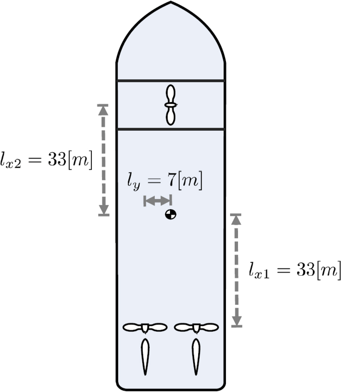
The control configuration of a ship

In this formulation, D₁ and D₂ represent the drag forces, while L₁ and L₂ represent the lift forces for the port and starboard rudder, respectively. The terms l_x1, l_x2 and l_y refer to the distances from the center of gravity to each propeller. The force generated by the propeller can be defined by the rotational speed n_i, and the thruster coefficient K_T with advance ratio J_i, as follows:

(6) Ti=KT(Ji)ρ|ni|niD4,i=1,2

where ρ denotes the density of water and D stands for the propeller's diameter. The tunnel thruster is also modeled using the rotational speed n₃, the propeller's diameter D₃, and the thruster coefficient K_T3 . However, it is important to note that the tunnel thruster can only generate sufficient force when the ship moves at low speeds. Consequently, we employ the tunnel thruster at lower speeds and model it with a constant thruster coefficient, independent of the advance ratio, as follows:

(7) T3=KT3ρ|n3|n3D34

The force exerted by a ship's rudder at low speed is notably influenced by the direction of the propeller's rotation. When the propeller rotates forward, ample lift is generated through propeller force and rudder angle interplay. However, generating effective lift is challenging when the propeller rotates in reverse. Consequently, the lift and drag forces produced by a pair of propellers and rudders can be formulated as follows, according to (Lindegaard, 2003):

(8) Li={TikLδδi,Ti≥00,Ti<0,i=1,2,Di={Ti(kDδ1|δi|+kDδ2δi2),Ti≥00,Ti<0,i=1,2.

Fig. 3 visually illustrates the force generated by a pair of propellers and rudders. Given that the ship's propellers and rudders can operate independently, the ship is viewed as a fully-actuated system capable of controlling motion across three degrees of freedom. Nevertheless, when considering the propulsion properties of the propellers and rudders, as demonstrated in Eq. (8), the system exhibits specific characteristics of being partially under-actuated.

Fig. 3.

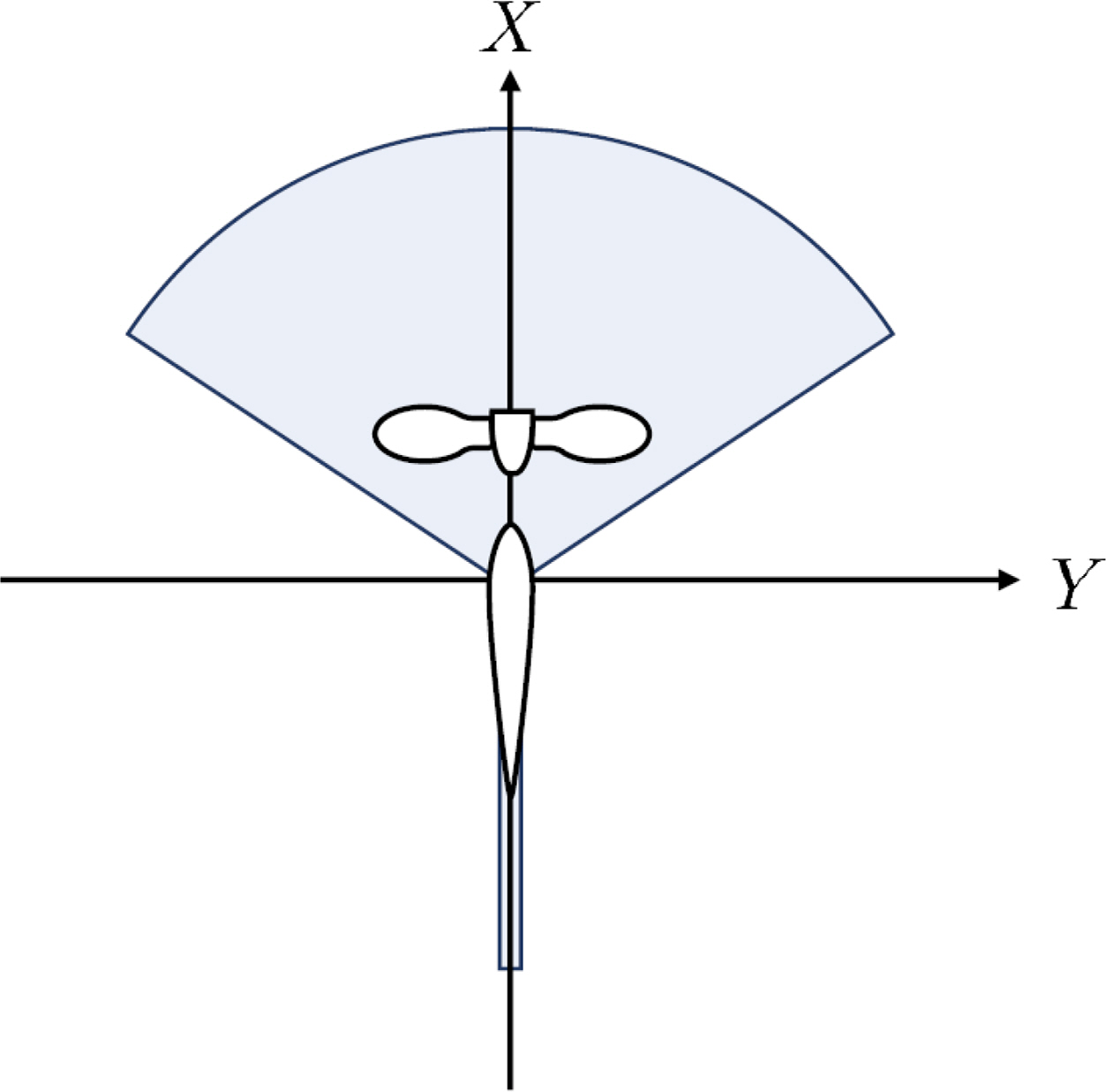
The feasible force domain of single-propeller, single-rudder

3. Berthing Trajectory Optimization

Given the initial and target berthing states, a trajectory optimization algorithm can be devised to minimize both the berthing duration and control effort, while taking into account the motion and control characteristics represented by Eqs. (1)–(8). However, the nonlinear nature and complexity of the optimization problem present a challenge in assuring optimal solutions. To tackle this issue, we propose an optimization approach that separates the trajectory into two distinct phases, thereby effectively reducing the complexity of the problem.

3.2 Two-point Boundary Value Problem

Employing models for each phase allows for the formulation of the two-point boundary value problem with the state vector x =[x,y,ψ,u,v,r]^⊤, as detailed below:

(11) minx(⋅),u(⋅)JT+∫0Tf1Ja(t)dt+JaTf1+∫Tf1Tf2Jt(t)dt

Here T_f1 and (T_f2 −T_f1) represent the time durations for each phase, respectively. Additionally, J_T denotes the time penalty cost function, which is defined as follows:

(12) JT(t)=ρt(Tf1+Tf2)

Here ρ_t is the weighting scalar. J_a(t), JaTf1 represent the cost functions for the approaching, which are defined as follows:

(13) Ja(t)=ν(t)⊤Qaν(t)+ua(t)⊤Paua(t)+u˙a(t)⊤Rau˙a(t)JaTf1=(η(Tf1)−ηf)⊤QaTf1(η(Tf1)−ηf)

In these equations, the matrices Q_a, P_a, and R_a denote the weight matrices that penalize the velocity, control input, and rate of change of control input, respectively. QaTf1 represents the weight matrix that penalizes the terminal position of the approaching phase, while η_f is the final position vector. Additionally, J_t (t) denotes the cost function for the terminal phase, given as follows:

(14) Jt(t)=ν(t)⊤Qtν(t)+ut(t)⊤Ptut(t)+u˙t(t)⊤Rtu˙t(t)

In this context, the matrices Q_t, P_t, and R_t represent the weight matrices that penalize the velocity, control input, and rate of change of control input, respectively. The optimization problem formulated above also encompasses several constraints, which are as follows:

(15) x˙(t)=fa(x(t),ua(t)),∀t∈[0,Tf1]x˙(t)=ft(x(t),ut(t)),∀t∈[Tf1,Tf2]x(0)=x0x(Tf2)=xf|u(t)|≤u(t)¯,∀t∈[0,Tf2]𝕊b⊆𝕊S

Here f_a and f_t represent the dynamic models of the approaching and terminal phases, respectively, while x₀ and x_f denote the initial and target berthing states. (⋅)¯ denotes the maximum value. The final constraints represent the collision avoidance condition. Here, 𝕊_b and 𝕊_s indicate the safety boundary of the ship and state constraints, as shown in Fig. 4.

Fig. 4.

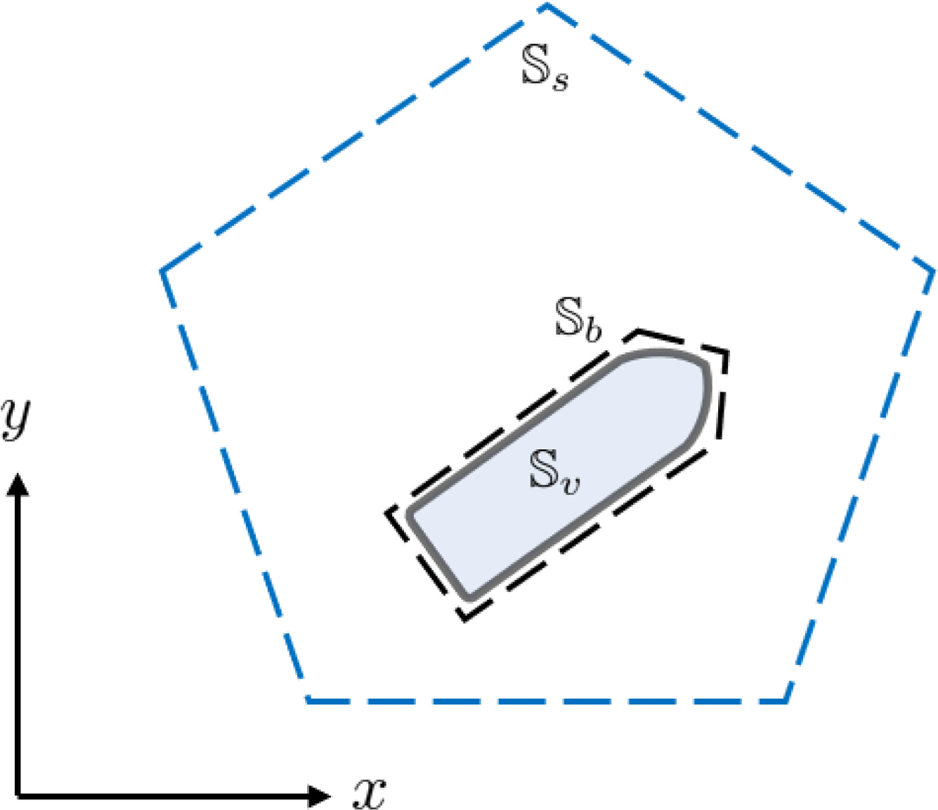
The illustration of collision avoidance constraints. (Ship 𝕊_v with a safety boundary 𝕊_b, as well as state constraints 𝕊_s)

To address the nonlinear optimization problem formulated in this manner, we utilized the Interior Point Optimizer (IPOPT) (Wächter and Biegler, 2006), implemented in the CasADI framework (Andersson et al., 2019), within the in the MATLAB environment.

4. Simulation Results

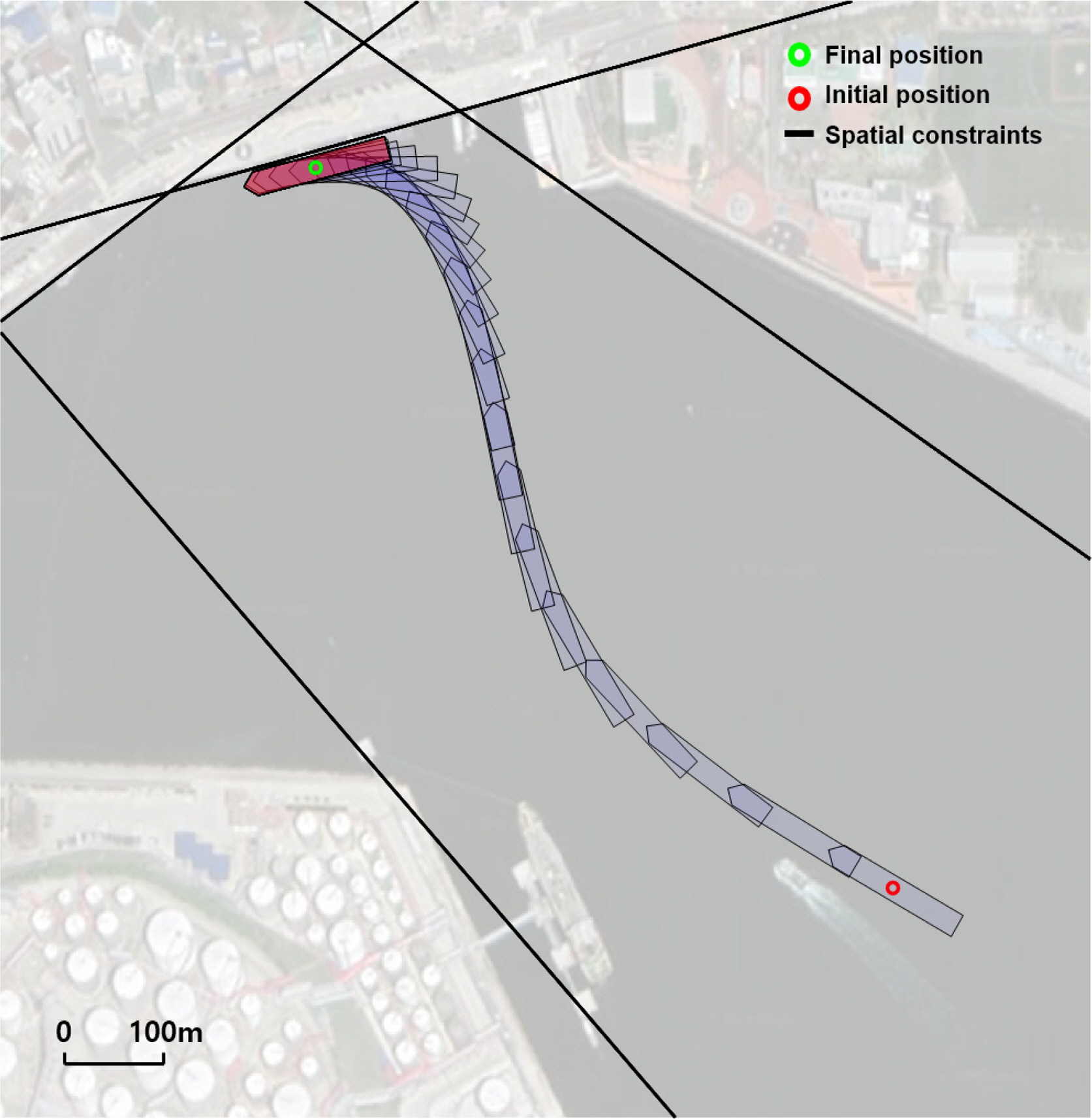
Simulations were executed within the MATLAB environment to evaluate the effectiveness of the proposed trajectory optimization algorithm. We incorporated the port geometry of Jangsaengpo Port in Ulsan, Korea, and devised two scenarios featuring distinct initial and final positions. The state constraints were formulated convexly, considering the berthing position, the port layout, and the ship's navigable area. It is worth noting that the specific configuration of these constraints can be altered based on the available space in the intended target port. The parameters of the supply ship's model used for simulation are derived from (Skjetne et al., 2004), with the remaining parameters detailed in Table 1. The parameters specific to our proposed algorithm can be found in Table 2. The results of the first simulation are visually represented in Figs. 5–7.

Table 1.

The model parameters of the ship

Table 2.

Parameters of the trajectory optimization problem

Fig. 5.

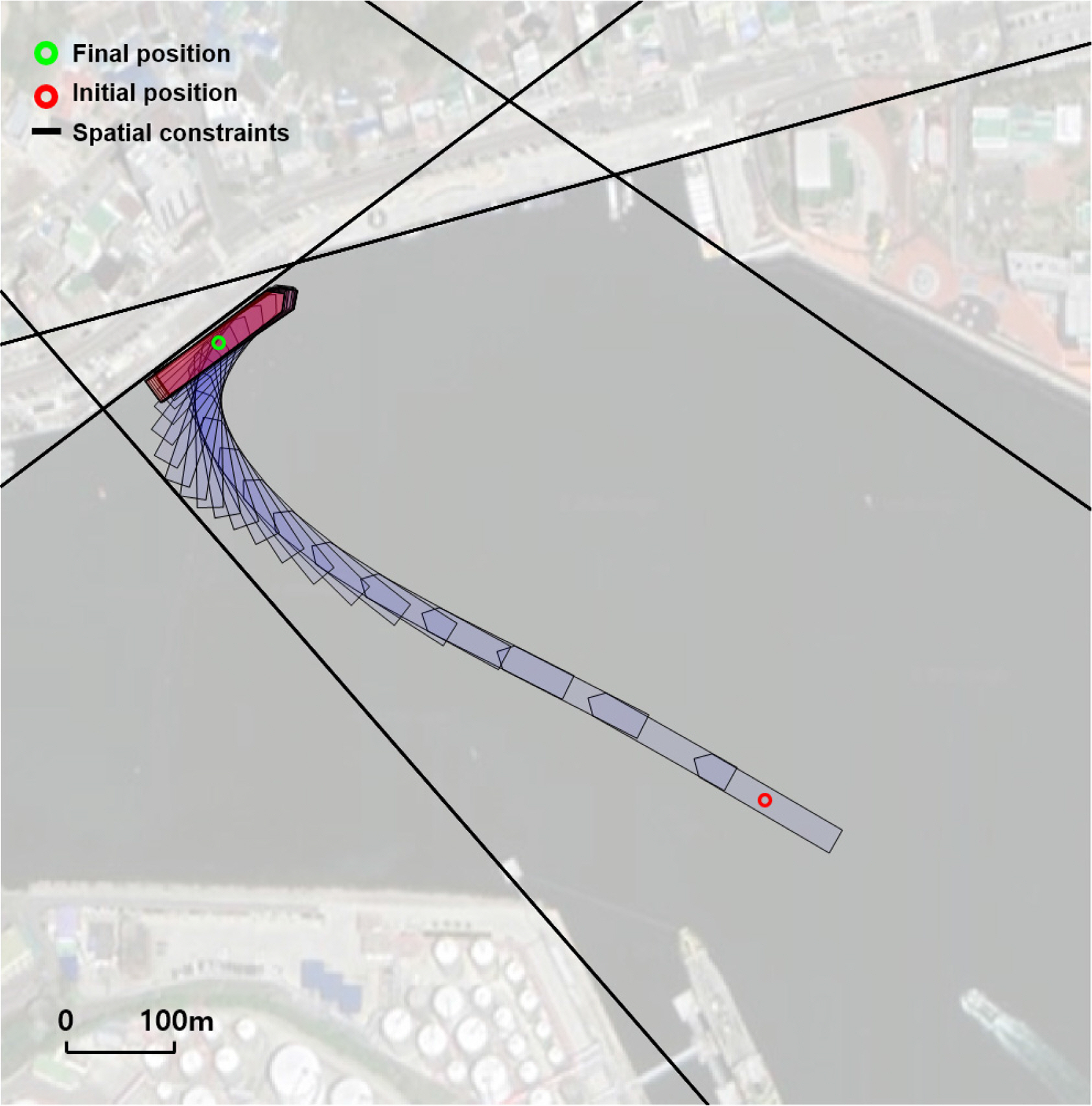
The result of the first scenario

Fig. 6.

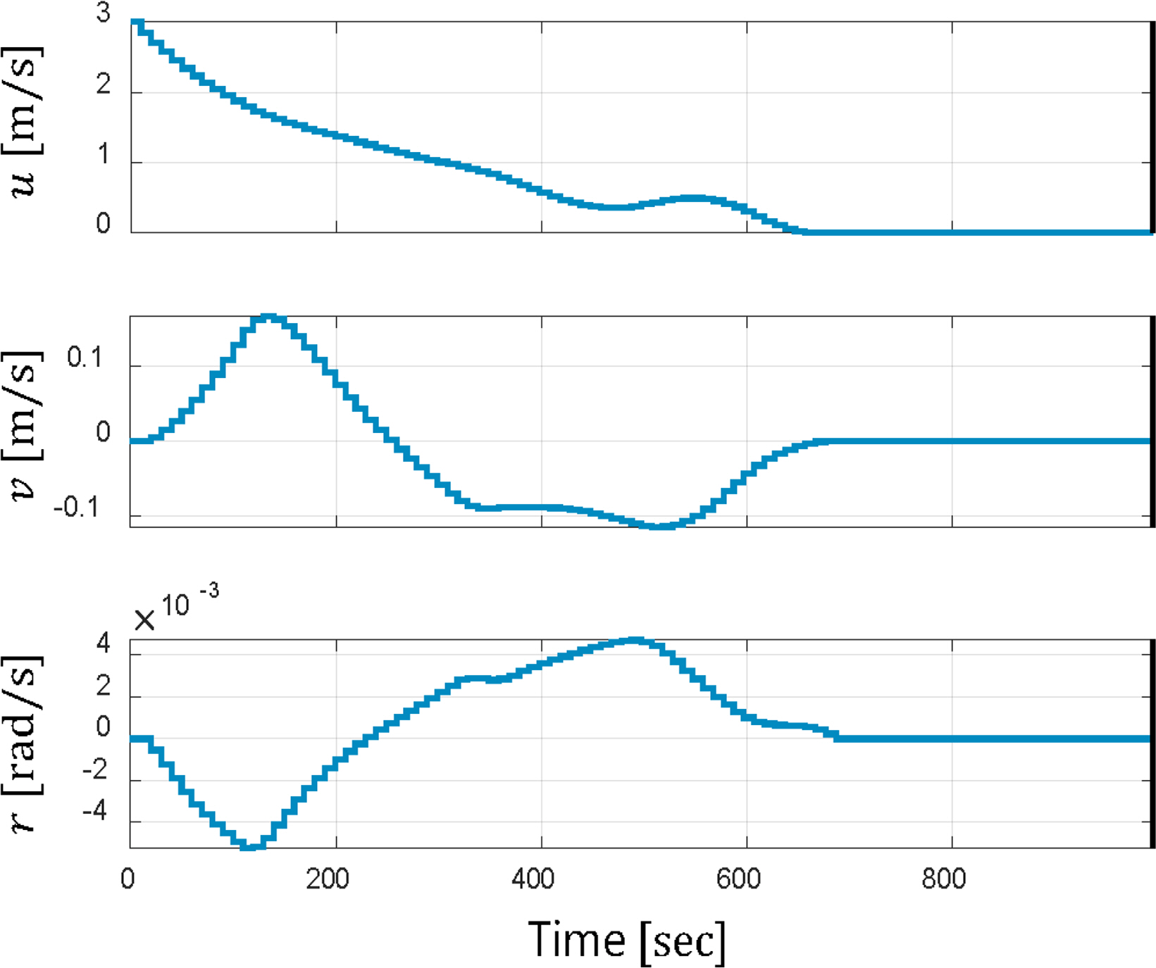
Time trajectories of velocities (first scenario)

Fig. 7.

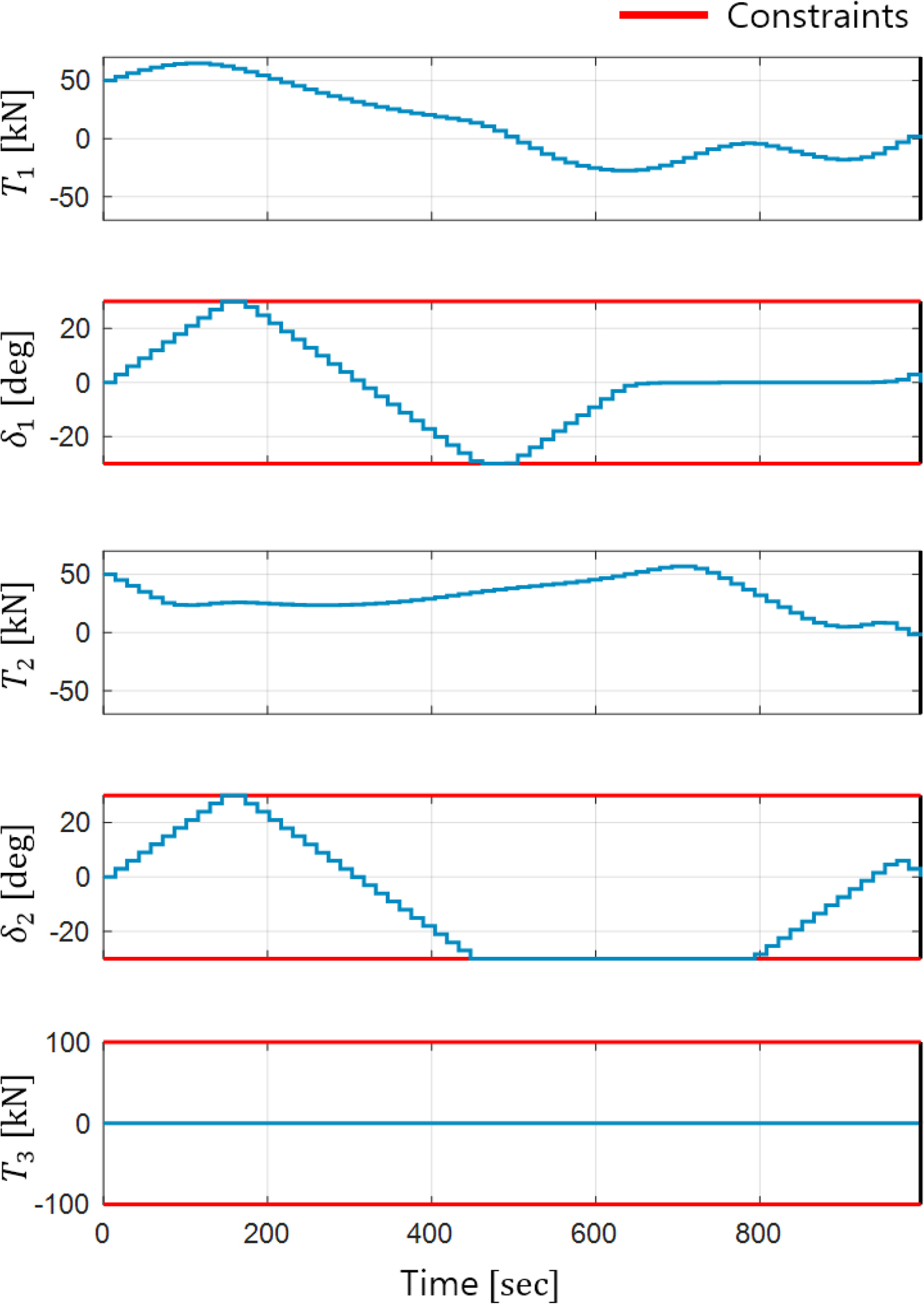
Time trajectories of control inputs (first scenario)

Fig. 5 illustrates the time trajectory for a port side berthing scenario. In this figure, the blue ship trajectory corresponds to the approaching phase, while the red ship trajectory represents the terminal phase. Fig. 6 illustrates the variation in velocities over the course of the berthing process, which lasts approximately 1026 seconds, with the approaching phase accounting for 940 seconds of this duration. This highlights a distinct phase switch. Fig. 7 shows the alterations in control input over time. These results corroborate that the proposed algorithm effectively considers the characteristic of not utilizing a rudder when the propeller is in reverse rotation.

In the second scenario, the objective is to berth a ship on the starboard side. The results of this simulation are depicted in Figs. 8–10. Fig. 8 displays the time trajectories for each phase. Figs. 9 and 10, on the other hand, portray the velocities and control input fluctuations over time, respectively. Contrary to the first scenario, the second scenario does not require a phase transition. This result arises from the optimization process determining that a sole emphasis on the approaching phase, without a phase transition, is more efficient for this scenario.

Fig. 8.

The result of the second scenario

Fig. 9.

Time trajectories of velocities (second scenario)

Fig. 10.

Time trajectories of control inputs (second scenario)

5. Conclusions

In this study, we have proposed a two-phase berthing trajectory optimization algorithm for the autonomous berthing of a twin-propeller, twin-rudder ship. The berthing process was segregated into two distinct phases, taking into account the ship's dynamic characteristics and actuator properties. We formulated models for each phase and generated dynamically feasible trajectories using a two- phase, two-point boundary value problem. To assess the practicality and effectiveness of our proposed algorithm, we created two scenarios grounded in real-world port geometries and conducted comprehensive numerical simulations.

Article information Continued