Analysis of Hydraulic Characteristics According to the Cross-Section Changes in Submerged Rigid Vegetation

Article information

J. Ocean Eng. Technol. 2022;36(5):326-339

Publication date (electronic) : 2022 October 28

doi : https://doi.org/10.26748/KSOE.2022.028

Jeongheum Lee ¹

, Yeon-Myeong Jeong ²

, Jun-Seok Kim ¹

, Dong-Soo Hur ³^,

¹Graduate Student, Department of Ocean Civil Engineering, Gyeongsang national University, Tongyeong, Korea

²Senior Researcher, Engineering Research Institute, Gyeongsang national University, Jinju, Korea

³Professor, Department of Ocean Civil Engineering, Gyeongsang national University, Tongyeong, Korea

Corresponding author Dong-Soo Hur: +82-55-772-9122, dshur@gnu.ac.kr

Received 2022 August 10; Revised 2022 August 26; Accepted 2022 August 28.

Abstract

Recently, not only Korea but also the world has been suffering from problems related to coastal erosion. The hard defense method has been primarily used as a countermeasure against erosion. However, this method is expensive and has environmental implications. Hence, interest in other alternative methods, such as the eco-friendly vegetation method, is increasing. In this study, we aim to analyze the hydraulic characteristic of submerged rigid vegetation according to the cross-sectional change through a hydraulic experiment and numerical simulation. From the hydraulic experiment, the reflection coefficient, transmission coefficient, and energy dissipation coefficient were analyzed according to the density, width, and multi-row arrangement of the vegetation zone. From numerical simulations, the flow field, vorticity distribution, turbulence distribution, and wave distribution around the vegetation zone were analyzed according to the crest depth, width, density, and multi-row arrangement distance of the vegetation zone. The hydraulic experiment results suggest that the transmission coefficient decreased as the density and width of the vegetation zone increased, and the multi-row arrangement condition did not affect the hydraulic characteristics significantly. Moreover, the numerical simulations showed that as the crest depth decreased, the width and density of vegetation increased along with vorticity and turbulence intensity, resulting in increased wave height attenuation performance. Additionally, there was no significant difference in vorticity, turbulence intensity, and wave height attenuation performance based on the multi-row arrangement distance. Overall, in the case of submerged rigid vegetation, the wave energy attenuation performance increased as the density and width of the vegetation zone increased and crest depth decreased. However, the multi-row arrangement condition did not affect the wave energy attenuation performance significantly.

Keywords: Submerged vegetation; Rigid vegetation; Laboratory experiment; Numerical wave tank; Hydraulic characteristics

1. Introduction

Recently, coastal erosion has become a major issue globally. Coastal erosion occurs owing to the rise in sea levels caused by global warming, invasion of high waves caused by abnormal temperatures, reduced soil supply caused by river development (e.g., dams), and change in the coastal environment caused by coastal development (e.g., port construction). When sand is lost owing to coastal erosion, the national land area decreases, thereby damaging those regions socially and economically . Countermeasures against coastal erosion include construction of gravity-based structures, such as groins and detached breakwaters, and beach nourishment. However, gravity-based structures are expensive and not eco-friendly, and beach nourishment is not a fundamental solution. Therefore, many studies have been conducted on countermeasures, and interest in the eco-friendly vegetation method has been increasing. While studies on vegetation have been conducted in the United States and Europe, such studies are not active in Korea.

Vegetation has different characteristics depending on various conditions, such as the shape of the material used, height of vegetation, and density and width of the vegetation zone, and many related studies were conducted on this topic (Anderso et al., 2011; Manca et al., 2010; Asano et al., 1988; Abdolahpour et al., 2017; Beudin et al., 2017; Hadadpour et al., 2019). Peruzzo et al. (2018) collected actual vegetation from nature and produced flexible vegetation with a similar shape. They performed a hydraulic model experiment and calculated the vegetation drag coefficient according to the density and depth of the vegetation zone. Wang et al. (2022) studied the wave transmission coefficient and drag coefficient of cylindrical flexible vegetation according to the depth and density through a hydraulic model experiment. Furthermore, various hydraulic model experiments on flexible vegetation have been performed (Blackmar et al., 2014; Maza et al., 2015). Additionally, Hu et al. (2014) studied wave height attenuation and the drag coefficient of vegetation according to the density and depth of the vegetation zone under the application of waves and flow for rigid cylindrical vegetation through a hydraulic model experiment. Van Veelen et al. (2020) performed a hydraulic model experiment on the effect of changes in the vegetation material on wave height attenuation and flow velocity using flexible and rigid vegetation with the same shape and size and different materials. Jeong and Hur (2016) developed a bidirectional coupled analysis technique by combining the discrete element method with the wave field model and numerically examined the wave attenuation effect according to the behavioral characteristics of vegetation.

As for submerged breakwaters, many studies have been conducted on the wave energy reduction effect by Bragg reflection that occurs when submerged breakwaters are arranged in multiple rows (Kirby and Anton, 1990; Cho et al., 2002; Cho, 2006). However, in the case of vegetation, studies on multi-row arrangement are insufficient.

In this study, a hydraulic model experiment and numerical model experiment were performed to analyze hydraulic characteristics according to the cross-section changes in submerged rigid vegetation. From the hydraulic model experiment, the hydraulic characteristics were analyzed according to the density and width of the vegetation zone and the cross-section change in multi-row arrangement. From the numerical model experiment, the flow field, vorticity distribution, turbulence distribution, and wave height distribution were analyzed according to the crest depth, density, width, and multi-row arrangement distance of the vegetation zone.

2. Hydraulic Model Experiment

2.1 Overview of the Hydraulic Model Experiment

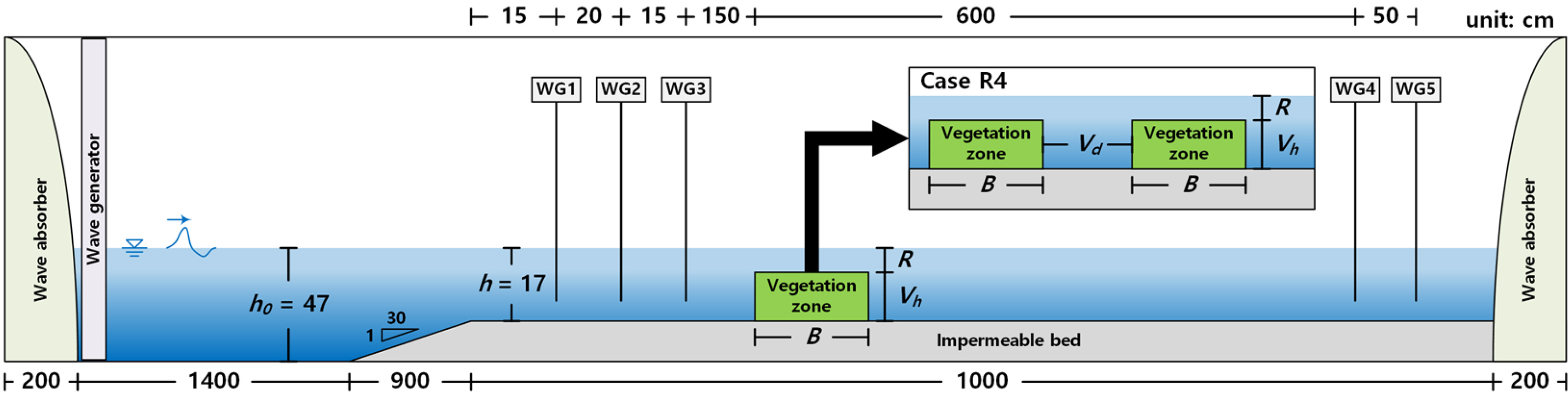
The hydraulic model experiment was performed to analyze hydraulic characteristics according to the cross-section variation in submerged rigid vegetation. A wave flume with a length of 37 m, height of 1 m, and width of 0.6 m was used in the experiment. A piston-type wave generator was used in the experiment. A 30 cm-high impermeable floor with a front inclination of 1:30 was constructed to generate waves, and a capacitance wave gauge was used to measure the wave height.

Fig. 1 and Table 1 show the configuration of the wave flume and the cross-section conditions of the vegetation. The density, width, and multi-row arrangement of the vegetation zone were considered for the cross-section conditions. The rigid vegetation used in the experiment was made of an acrylic material, as shown in Fig. 2(a). Fig. 3 shows the frame fixed vegetation. Figs. 3(a) and 3(b) represent cases in which the vegetation densities (ρ_V) are 0.123 and 0.032, respectively.

(1) S(f)=0.257HS2TS−4f−5exp[−1.03(TSf)−4]

where S (f) is the wave spectral density, H_S is the significant wave height, T_S is the significant wave period, and f is the frequency.

Fig. 1.

Sketch of wave flume and experimental setup

Table 1.

Vegetation cross section condition

Fig. 2.

Vegetation used in the experiment: (a) specification of vegetation; (b) vegetation zone installed in the wave flume

Fig. 3.

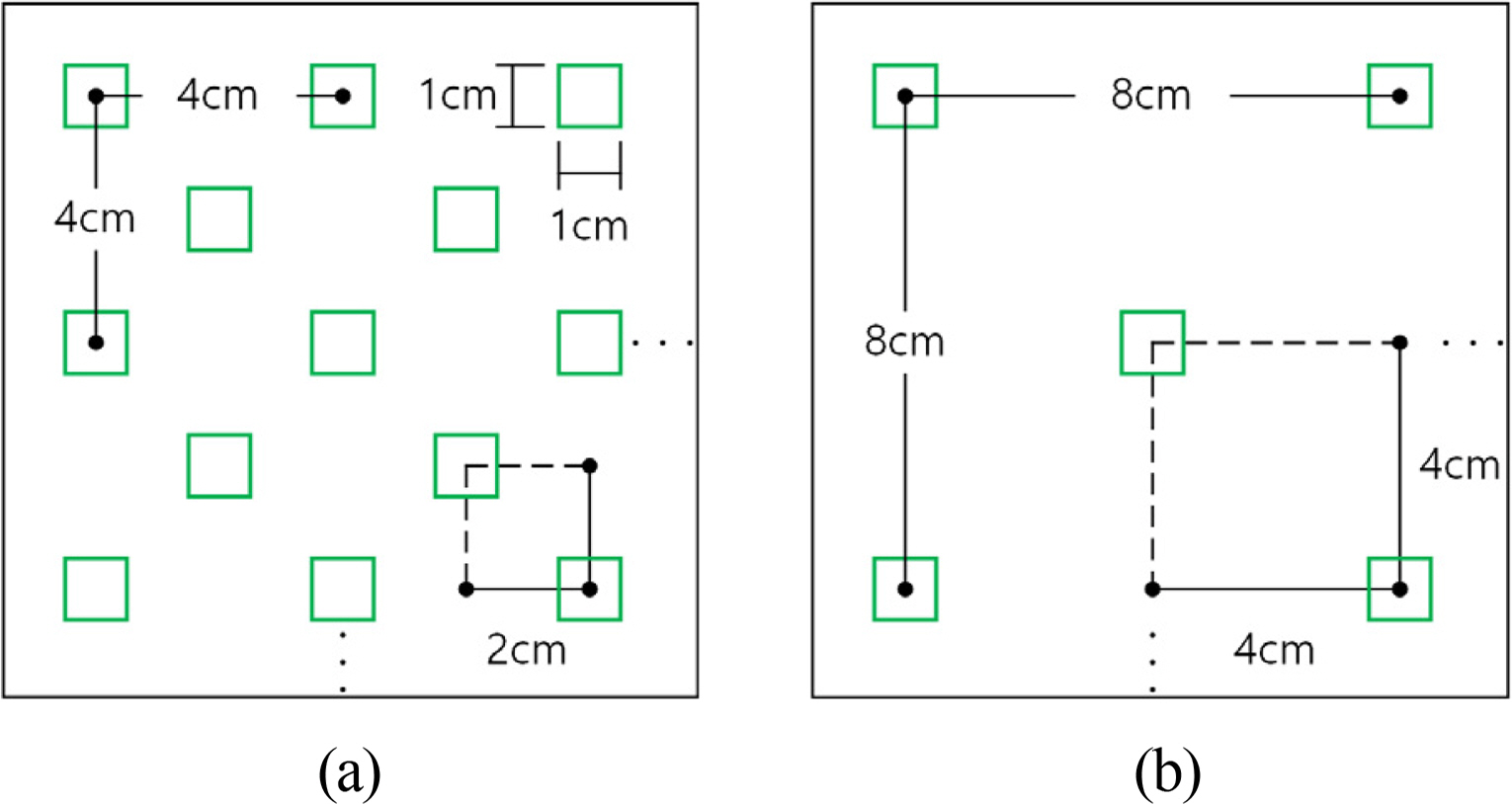
Sketch of frame fixed vegetation: (a) ρ_V = 0.123; (b) ρ_V = 0.032

Table 2 shows the incident wave conditions. The incident waves were irregular waves with a wave height of 2.67‒11.0 cm and a period of 0.64–1.88 s. The Bretschneider–Mitsuyasu spectrum of Eq. (1) proposed by Mitsuyasu (1969) was used to generate the irregular waves. In Fig. 4, the theoretical values of the Bretschneider–Mitsuyasu spectrum are compared with those obtained from the experiment. Figs. 4(a) and 4(b) represent wave case 4 (H_S = 5.33 cm, T_S = 0.95 s) and wave case 16 (H_S = 11.0 cm, T_S = 1.88 s), respectively.

Table 2.

Incident wave condition (wave type = irregualar, h = 17 cm)

Fig. 4.

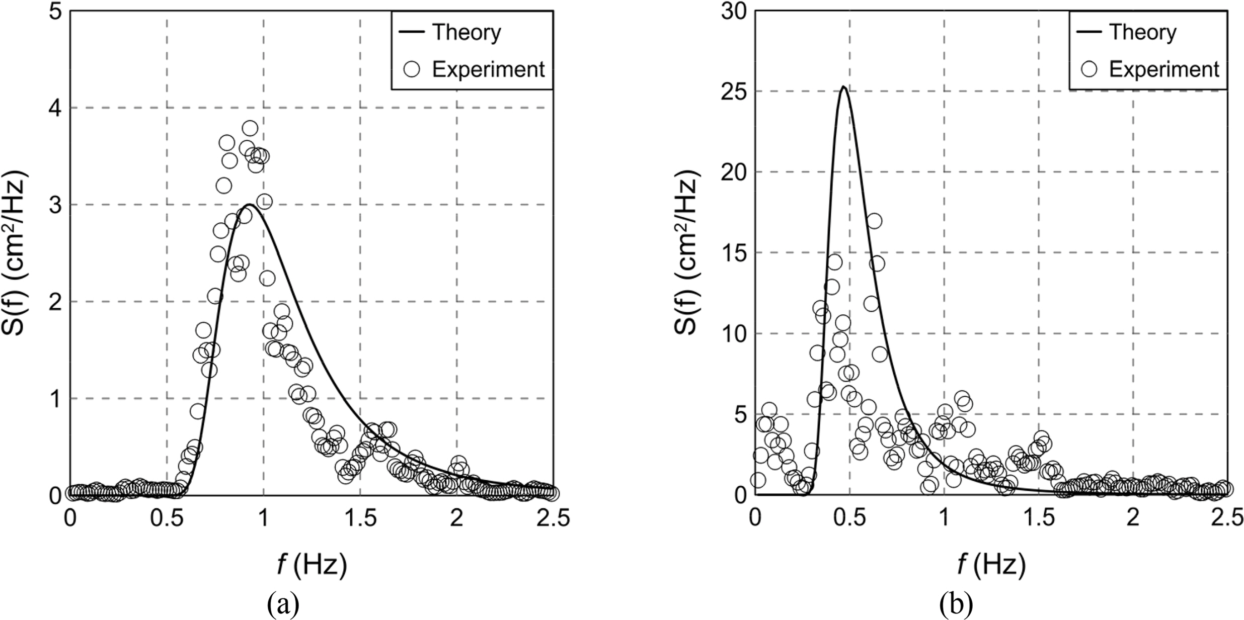
Comparison between theoretical and experimental spectra: (a) wave case 4; (b) wave case 16

The reflection coefficient (K_R), transmission coefficient (K_T), and energy dissipation coefficient (K_D) were calculated to analyze hydraulic characteristics according to the cross-section changes in submerged rigid vegetation. The reflection coefficient (K_R) was calculated using the incident/reflected wave separation method proposed by Goda and Suzuki (1976). The transmission coefficient (K_T) and energy dissipation coefficient (K_D) were calculated using Eqs. (2) and (3), respectively.

(2) KT=HTHO

where H_O is the incident wave height and H_T is the transmitted wave height.

(3) KD=1−KR2−KT2

2.2 Results of the Hydraulic Model Experiment

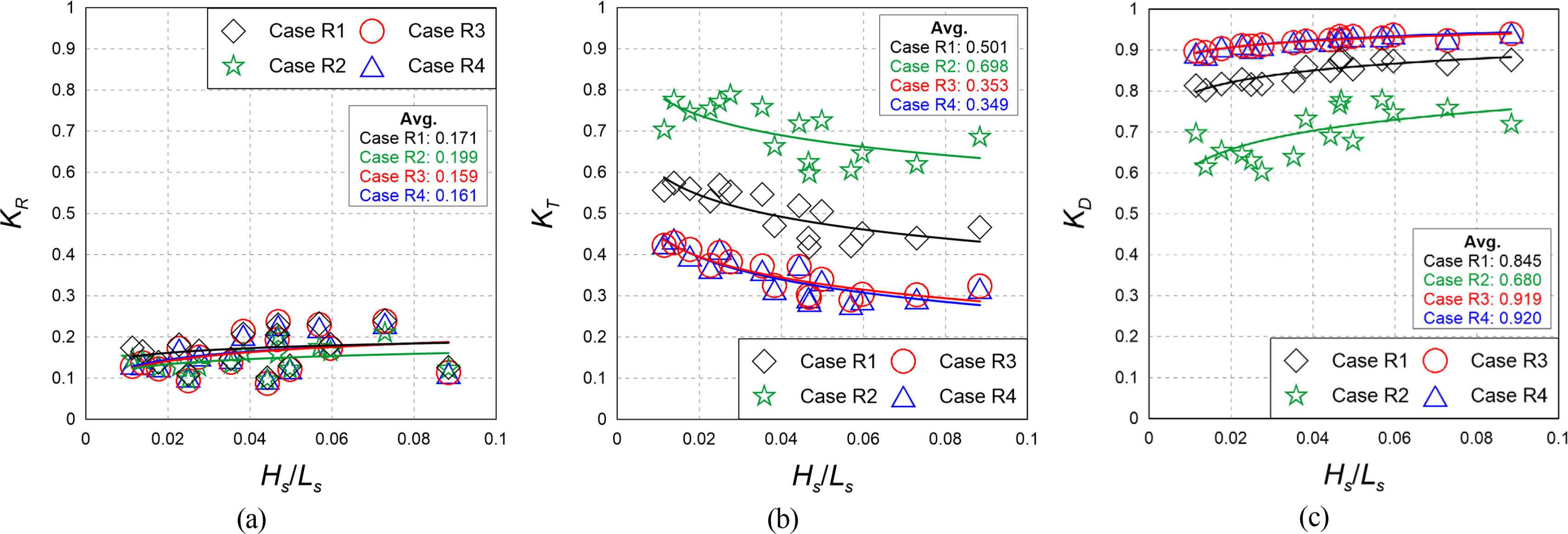
A fixed-bed hydraulic model experiment was performed as a preliminary experiment to examine the hydraulic characteristics of wave propagation according to the cross-section changes in submerged rigid vegetation. In other words, K_R, K_T, and K_D were calculated according to the density, width, and multi-row arrangement conditions of submerged rigid vegetation. Fig. 5 shows the distribution of the coefficients according to the wave steepness. Figs. 5(a), 5(b), and 5(c) represent the cases of K_R, K_T, and K_D, respectively.

Fig. 5.

Comparison of K_R, K_T, and K_D according to changes in the cross-section condition of the rigid vegetation zone

2.2.1 Reflection coefficient

The reflection coefficient was not significantly different depending on the width and multi-row arrangement for Case R1 (B = 133 cm, ρ_V = 0.123), Case R3 (B = 266 cm, ρ_V = 0.123), and Case R4 (B = 133, 133 cm, ρ_V = 0.123), which had the same density. It decreased slightly for Case R2 (B = 133 cm, ρ_V = 0.032), which had lower density. This is because the reflected wave was generated similarly when the density of the vegetation zone was the same and the transmission area of waves increased as the vegetation density decreased.

2.2.2 Transmission coefficient

The transmission coefficient was found to decrease in Case R3 (B = 266 cm, ρ_V = 0.123) and Case R4 (B = 133, 133 cm, ρ_V = 0.123), where the density was the same and the width of the vegetation zone increased compared to that in Case R1 (B = 133 cm, ρ_V = 0.123), and in Case R2 (B = 133 cm, ρ_V = 0.032), where the width was identical and the density decreased. This is because an increase in the density and width of the vegetation zone induces more breaking waves at the crest of the vegetation zone.

2.2.3 Energy dissipation coefficient

The energy dissipation coefficient was the lowest in Case R2 (B = 133 cm, ρ_V = 0.032), where the width and density of the vegetation zone were low, and showed a tendency to increase as the width and density of the vegetation zone increased. Additionally, there was no significant difference in hydraulic characteristics between Case R3 (B = 266 cm, ρ_V = 0.032) and Case R4 (B = 133, 133 cm, ρ_V = 0.032), which had the same density and width of the vegetation zone. In the case of submerged rigid vegetation, it was assumed that the multi-row arrangement condition does not affect the wave energy attenuation of the incident wave significantly.

3. Overview of the Numerical Model Experiment

The numerical model experiment was performed to analyze hydraulic characteristics according to the cross-section changes in the submerged rigid vegetation. As for the numerical model, LES-WASS-2D (Hur and Choi, 2008), a complete nonlinear two-dimensional (2D) model that can consider the energy dissipation by fluid resistance according to the characteristics of the permeable medium based on the porous body model and volume of fluid capable of considering the effect of permeability, was used.

3.1 Governing Equations

The basic equations of the numerical model consist of the continuity equation, modified Navier–Stokes equations, and advection equation, which are shown in Eq. (4), Eqs. (5)–(6), and Eq. (7), respectively.

(4) ∂(γxu)∂x+∂(γzw)∂z=q*

(5) γv∂u∂t+u∂(γxu)∂x+w∂(γzu)∂z =−γv1ρ∂p∂x+1p[∂∂x{γxνt(2∂u∂x)}+∂∂z{γ2νt(∂u∂z+∂w∂x)}] −Mx−Ex−Dx

(6) γv∂w∂t+u∂(γxw)∂x+w∂(γzw)∂z =−γz1ρ∂p∂z+1p[∂∂x{γxνt(∂w∂x+∂w∂z)}+∂∂z{γ2νt(2∂w∂z)}] −2ν3∂q*∂z−γvg−βw−Mz−Ez−Dz

(7) ∂(γvF)∂t+∂(γxFu)∂x+∂(γzFw)∂z=Fq*

where u and w are the flow velocities in the x and z directions, respectively. q^* is the flow density of the wave source. M_x and M_z are inertial resistance. E_x and E_z are laminar flow resistance. D_x and D_z are turbulence resistance. γ_v is the volumetric porosity. γ_x and γ_z are the area permeabilities along the x and z directions, respectively. t is the time, g is the gravitational acceleration, ρ is the fluid density, p is the pressure, β is the wave attenuation coefficient, F is the volume ratio occupied by the fluid in each grid, and ν_t is the sum of the kinematic viscosity coefficient and kinematic eddy viscosity.

3.2 Vegetation Drag

The fluid resistance by vegetation (RV_i) is given by Eq. (8).

(8) RVi=12CDΦvivi2+vj2+CM(1−γv)∂vi∂t

where Φ is the vegetation density, C_D is the drag coefficient, and C_M is the inertial resistance.

For C_D, Eq. (9), which was presented by Lee et al. (2017a) by analyzing the experimental results of Wu and Cox (2015), was applied. C_M = 1.5, as proposed by Sakakiyama and Kajima (1992), was applied.

(9) CD=1.4(1+15KC)

where KC is the Keulegan–Carpenter number.

3.3 Verification of the Numerical Wave Tank

To examine the validity of the numerical model, a 2D numerical wave tank was constructed, as shown in Fig. 6. The lengths of the x and z axes were set to be 1000 and 30 cm, respectively. The grid sizes of Δx and Δz were set to be 1 cm. Additional dissipation zones were prepared at both ends of the tank to prevent the reflection and re-reflection of waves.

Fig. 6.

Sketch of the numerical wave tank based on the hydraulic experiment

The numerical wave tank was compared and verified for the experimental conditions shown in Table 3 for the wave and vegetation cross-section conditions applied in the hydraulic model experiment. As the planar arrangement of rigid vegetation could not be reproduced owing to the characteristics of the 2D numerical model, the vegetation density was replaced with porosity in the numerical model.

Table 3.

Conditions of incident waves and vegetation cross-section used in this study

In Fig. 7, the results of the hydraulic and numerical model experiments are compared. Figs. 7(a), 7(b), and 7(c) represent the reflection coefficient, transmission coefficient, and energy dissipation coefficient, respectively. For the reflection and transmission coefficients, the calculation results tended to be slightly higher than the experimental values when the wave steepness was low (near H_S/L_S = 0.02). Overall, it was assumed that the calculated values reproduced the experimental values properly. In Fig. 8, the dotted lines show the ±10% range of the values of the hydraulic and numerical model experiments. Overall, it can be seen that the results of the numerical model experiment reproduced the reflection coefficient, transmission coefficient, and energy dissipation coefficient of the hydraulic model experiment appropriately.

Fig. 7.

Comparison of reflection, transmission, and energy dissipation coefficients between the experimental and calculated values

Fig. 8.

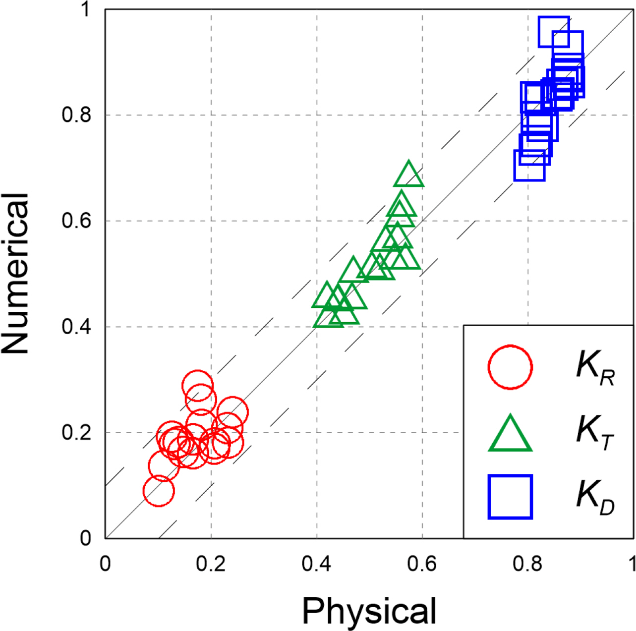
Comparison of K_R, K_T, and K_D between the experimented and calculated values

4. Results of the Numerical Model Experiment

For a closer analysis of the hydraulic characteristics according to the cross-section changes in submerged rigid vegetation, which were examined in the numerical model experiment, the flow field, vorticity distribution, turbulence distribution, and wave height distribution around the submerged rigid vegetation were examined using the validated numerical wave tank. As shown in Fig. 6 and Table 4, additional experimental conditions compared to the hydraulic model experiment were applied to the numerical wave tank. A regular wave was used as the incident wave to facilitate the analysis. Additionally, the crest depth (R), width (B), density (ρ_V), and arrangement distance (V_d) were considered for the cross-section conditions of the vegetation zone.

Table 4.

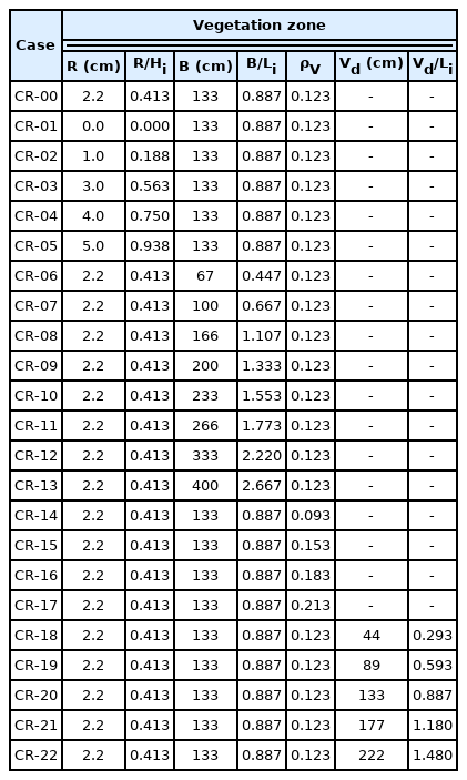
Experimental conditions used in this study (wave conditions: H_i = 5.33 cm, T_i = 1.26 s)

The vorticity was calculated using Eqs. (10)–(14), which were proposed by Raffel et al. (1998) and Raffel et al. (2007) as in Lee et al. (2017b). Positive (+) values in red represent the counterclockwise direction and negative (−) values in blue represent the clockwise direction.

(10) ωxz=(ΩA+ΩB−ΩC−ΩD)4ΔxΔz

(11) ΩA=12Δx(ui−1,k−1+2ui,k−1+ui+1,k−1)

(12) ΩB=12Δz(wi+1,k−1+2wi+1,k+wi+1,k+1)

(13) ΩC=12Δx(ui+1,k+1+2ui,k+1+ui−1,k+1)

(14) ΩD=12Δz(wi−1,k+1+2wi−1,k+wi−1,k−1)

In the case of turbulence, turbulence with a relatively large structure was calculated directly. For turbulence smaller than the grid size, the large eddy simulation technique that utilizes the sub-grid scale (SGS) model was used, and the Smagorinsky SGS model (Smagorinsky, 1963) expressed using the following equations was used.

(15) νt=ν+νl

(16) νl=(CSΔ)2|S|

(17) |S|=(2SijSij)1/2

(18) Sij=12(∂ui∂xj+∂uj∂xi)

(19) Δ=(ΔxΔz)1/2

where ν is the kinematic viscosity coefficient, ν_l is the kinematic eddy viscosity of SGS, ∆ is the filter length scale, and S_ij is the deformation tensor at the grid size. As for the C_S value, Schumann (1987) proposed a value ranging from 0.07 to 0.21, but 0.1 was used in this study because it was applied in a similar study (Christensen and Deigaard, 2001; Okayasu et al., 2005).

4.1 Flow Field, Vorticity Distribution, Turbulence Distribution, and Wave Height Distribution According to the Crest Depth

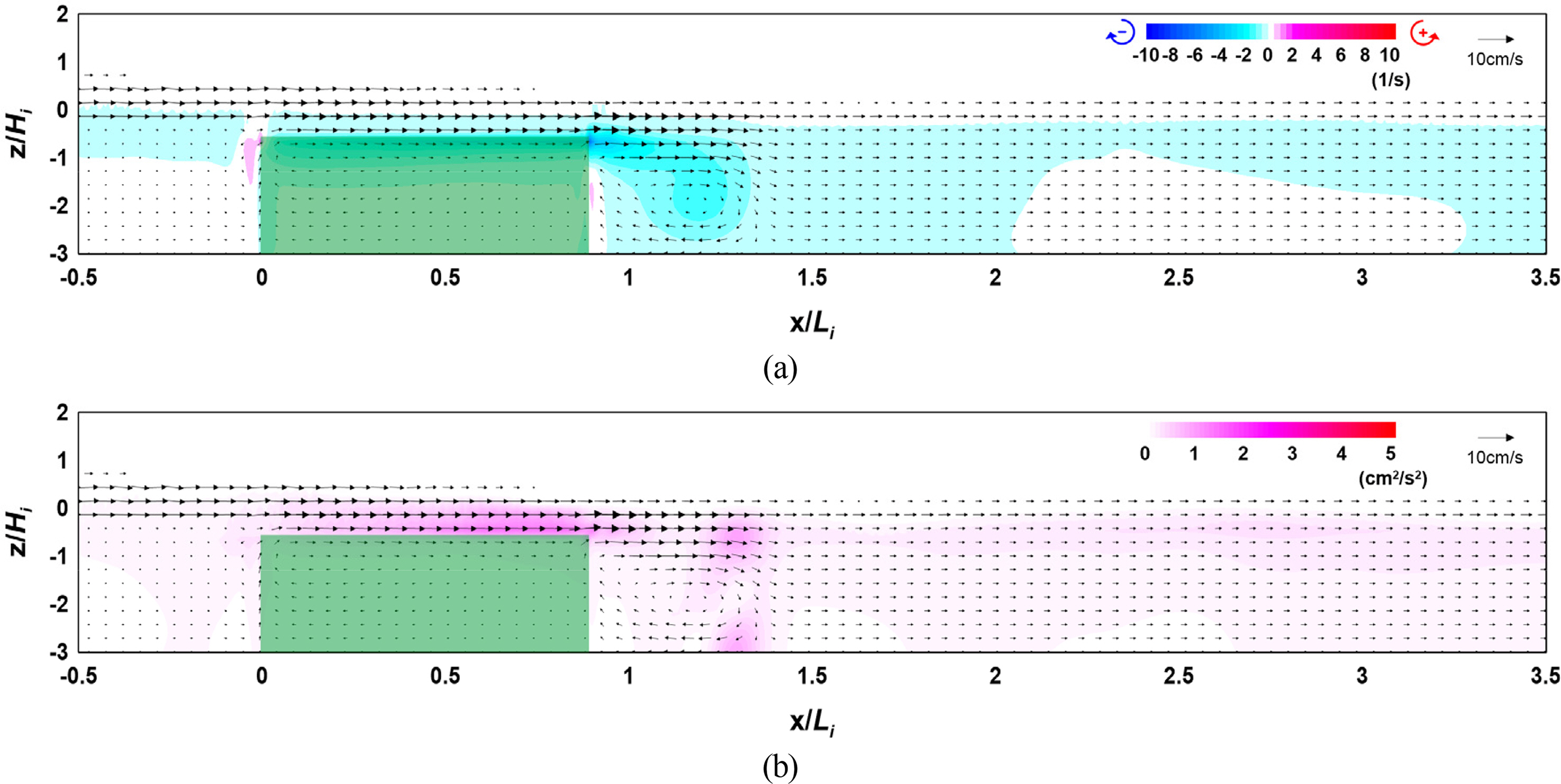
Figs. 9 and 10 show the flow field, vorticity distribution, and turbulence distribution according to the crest depth of the vegetation zone. Fig. 11 shows the wave height distribution around the submerged rigid vegetation according to the crest depth. From Figs. 9 and 10(a), clockwise (−) and counterclockwise (+) vortices can be confirmed in the vorticity distribution around the rigid vegetation. Additionally, a strong vorticity distribution is formed in the clockwise direction behind the vegetation, and the case of Fig. 9(a) with a low crest depth shows a stronger and wider vorticity distribution than the case of Fig. 10(a).

Fig. 9.

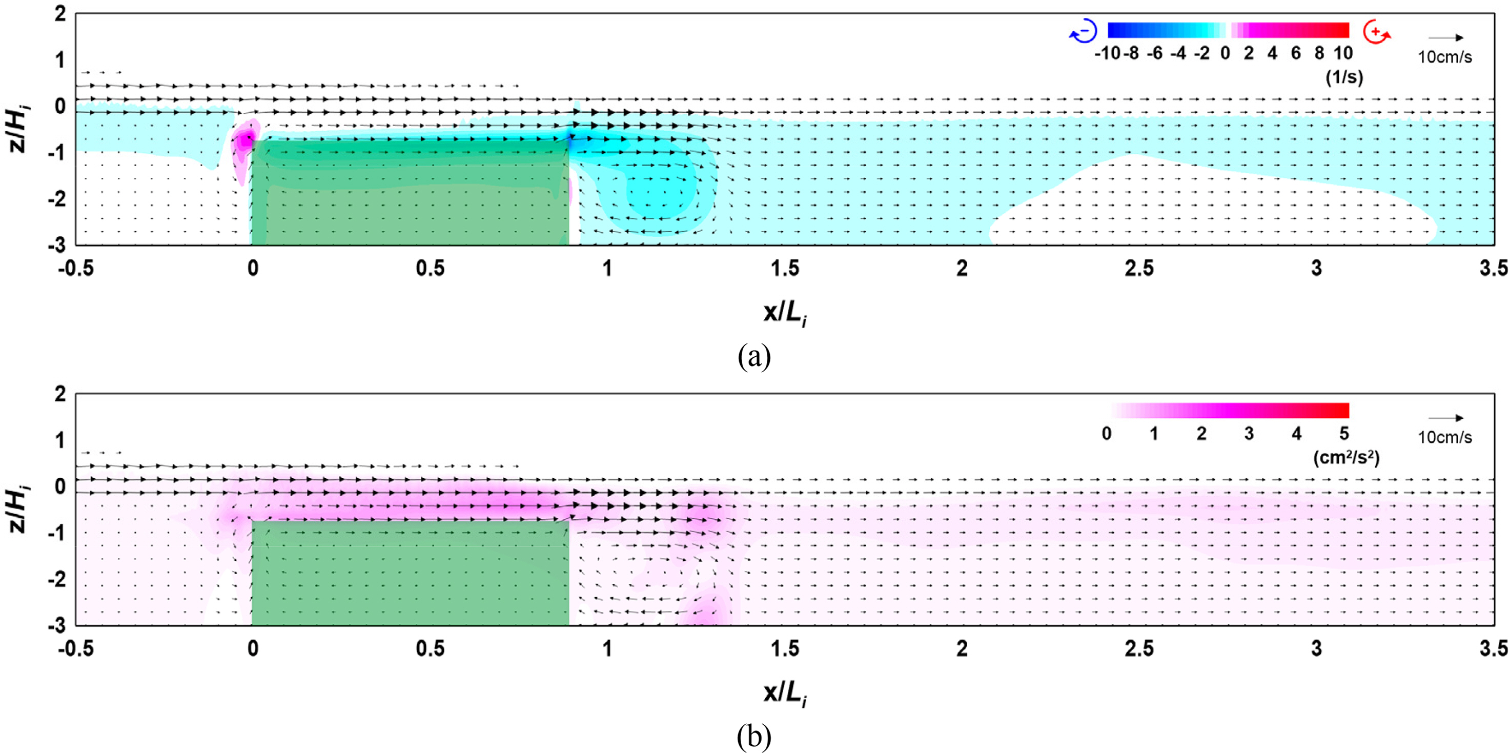
Flow field, vorticity distribution, and turbulence distribution around the vegetation (Case CR-03, R/H_i = 0.563): (a) flow field and vorticity distribution; (b) flow field and turbulence distribution

Fig. 10.

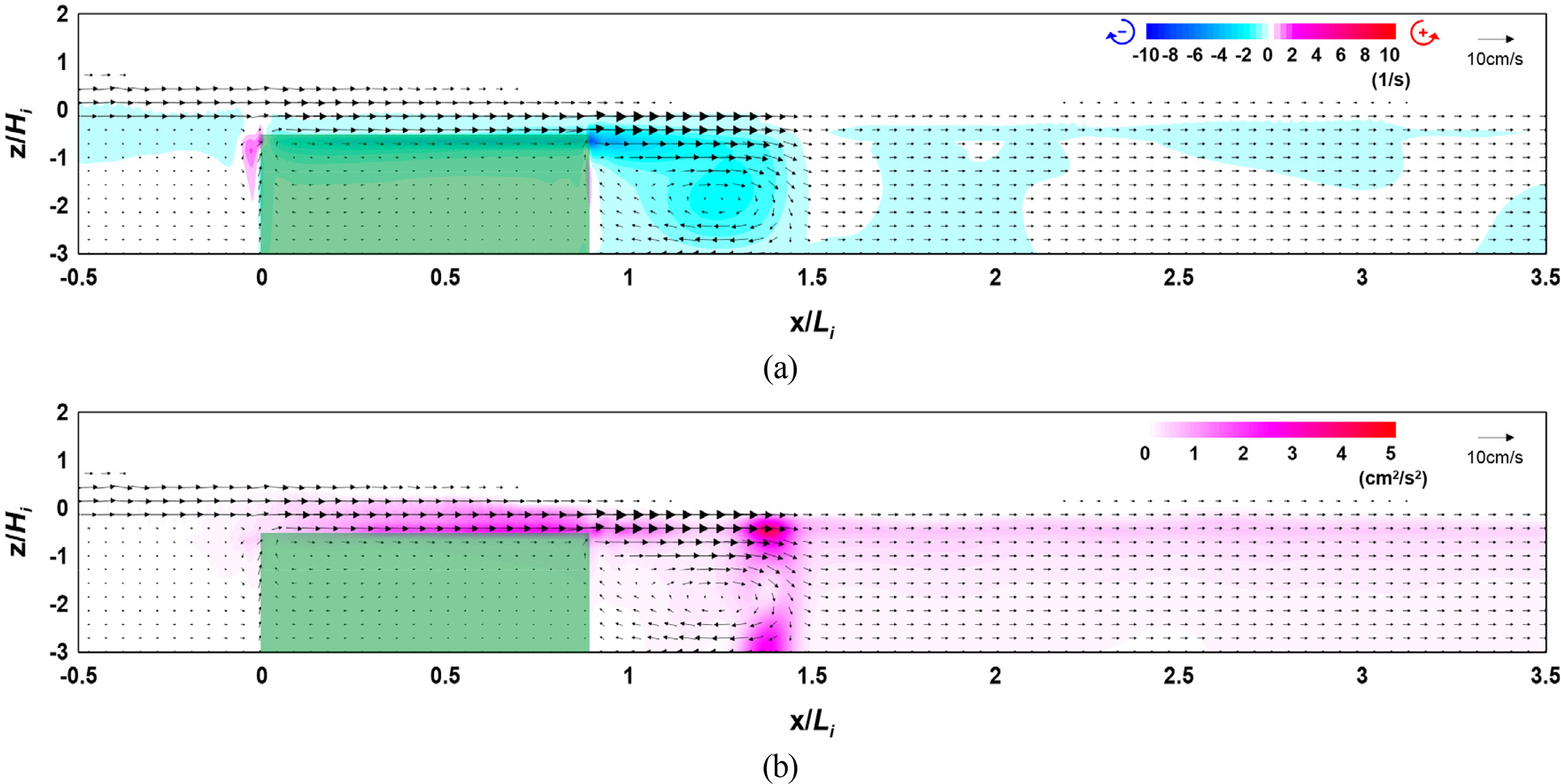
Flow field, vorticity distribution, and turbulence distribution around the vegetation owing to the ridge (Case CR-05, R/H_i = 0.938): (a) flow field and vorticity distribution; (b) flow field and turbulence distribution

Fig. 11.

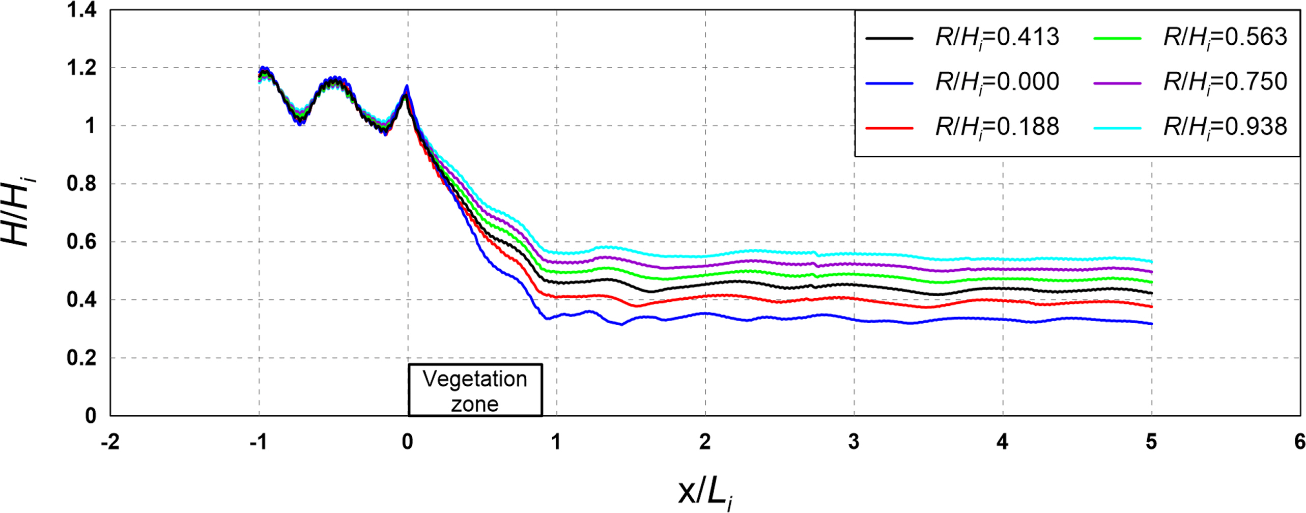
Wave height distribution according to changes in crest depth of the vegetation zone (R/H_i)

Figs. 9 and 10(b) show that a large turbulence distribution is formed at the crest and back of the submerged vegetation. This is because strong flow velocity corresponding to breaking waves occurs on the crest of the rigid vegetation. Additionally, the turbulence intensity on the crest of the rigid vegetation is higher and the turbulence distribution behind the rigid vegetation is wider in the case of Fig. 9(b). However, the crest depth was lower than that shown in the case of Fig. 10(b).

In Fig. 11, it can be seen that a slight partial standing wave field is formed in front of the submerged rigid vegetation under the influence of the reflected waves by the vegetation, and the height of waves that pass through the vegetation is reduced at the back by the energy dissipation caused by the resistance of the vegetation. This wave height attenuation effect tended to increase as the crest depth decreased as with the characteristics of typical submerged breakwaters.

4.2 Flow Field, Vorticity Distribution, Turbulence Distribution, and Wave Height Distribution According to the Width

Figs. 12 –14 show the flow field, vorticity distribution, and turbulence distribution according to the width of the vegetation zone. Fig. 15 shows the wave height distribution around the submerged vegetation according to the width. From Figs.. 12(a), 13(a), and 14(a), it can be seen that the flow velocity decreases as the width of the vegetation zone increases owing to a reduction in waves that propagate onto the vegetation crest, thereby forming a strong clockwise vorticity distribution behind the submerged vegetation. From Figs. 12(b), 13(b), and 14(b), it can be seen that a large turbulence distribution is formed at the crest and back of the submerged vegetation, and that the turbulence intensity behind the vegetation zone increases as the width of the zone increases. Therefore, the increasing wave height attenuation effect alongside the increase in the width of the submerged vegetation can be confirmed by the wave height distribution shown in Fig. 15.

Fig. 12.

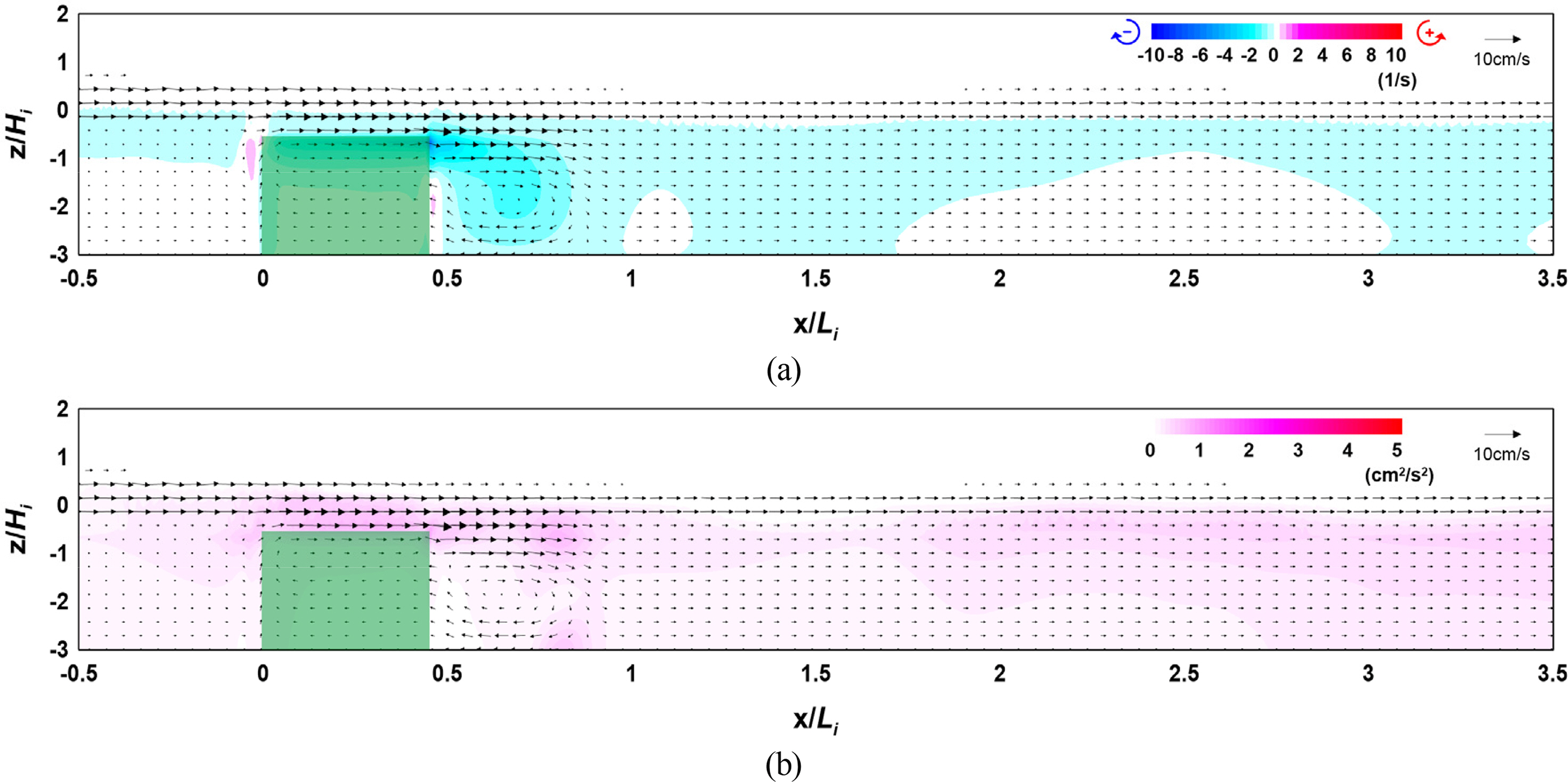
Flow field, vorticity distribution, and turbulence distribution around the vegetation (Case CR-06, B/L_i = 0.447): (a) flow field and vorticity distribution; (b) flow field and turbulence distribution

Fig. 13.

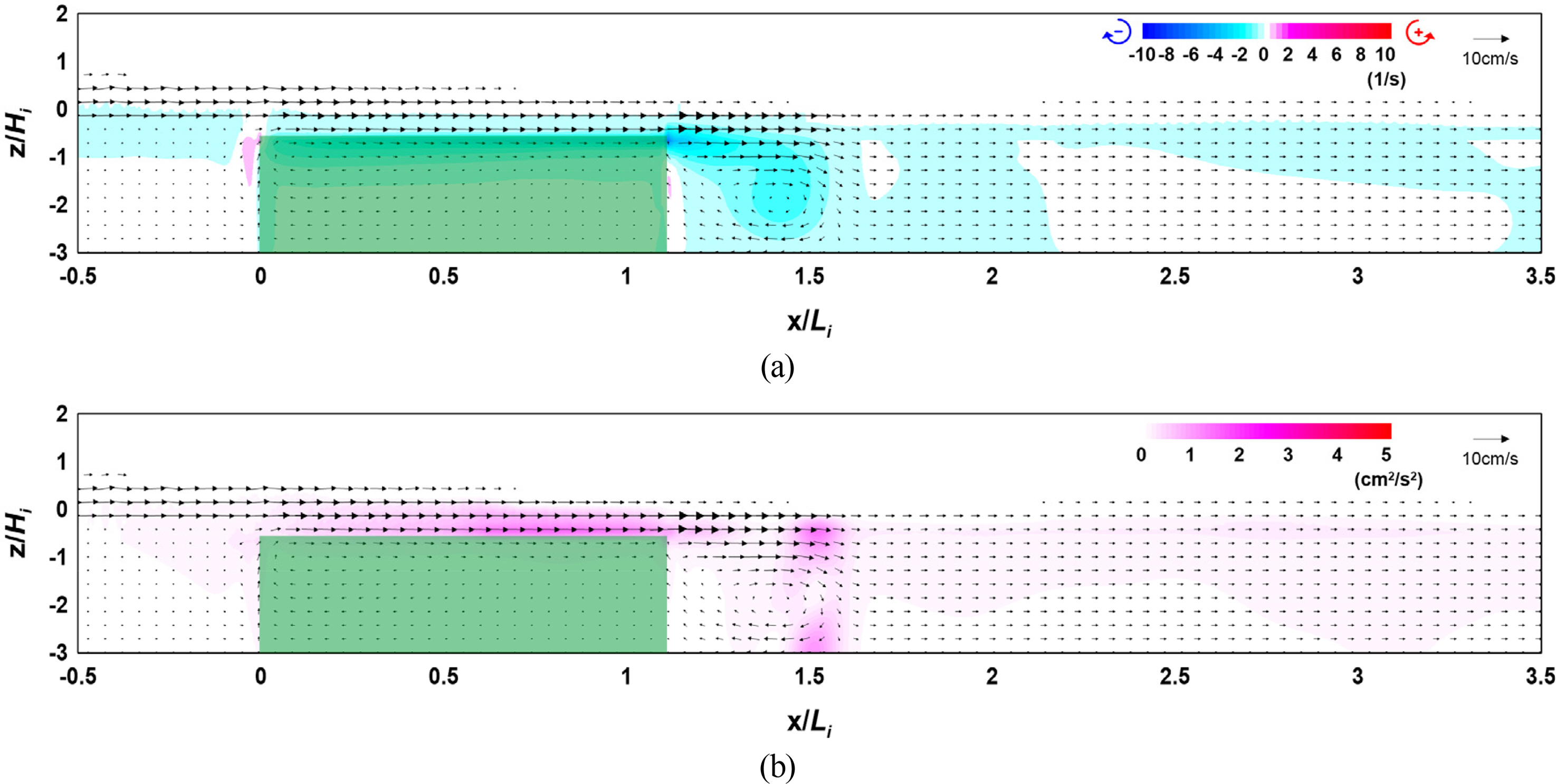
Flow field, vorticity distribution, and turbulence distribution around the vegetation (Case CR-08, B/L_i = 1.107): (a) flow field and vorticity distribution; (b) flow field and turbulence distribution

Fig. 14.

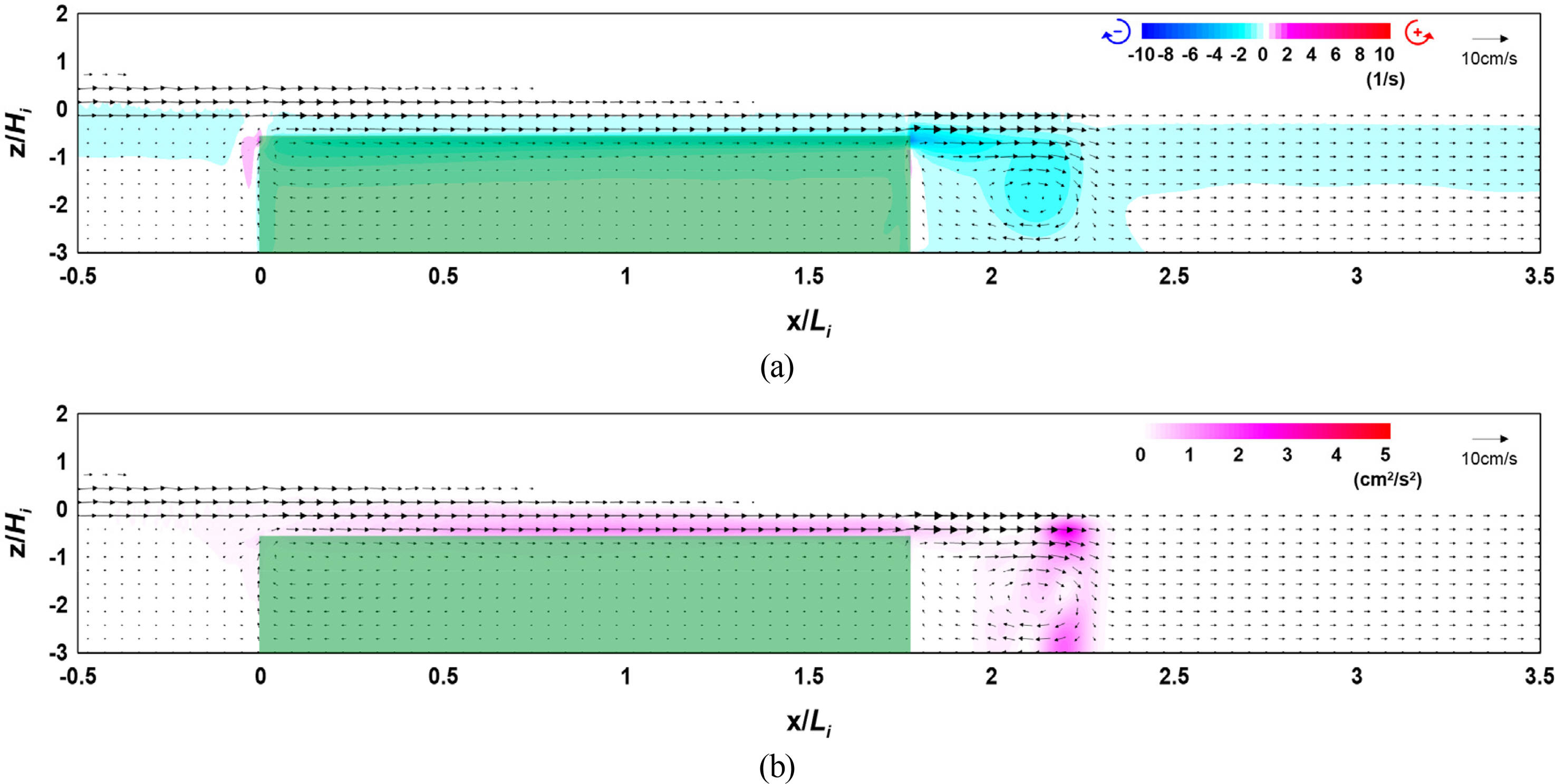
Flow field, vorticity distribution, and turbulence distribution around the vegetation (Case CR-11, B/L_i = 1.773): (a) Flow field and vorticity distribution; (b) Flow field and turbulence distribution

Fig. 15.

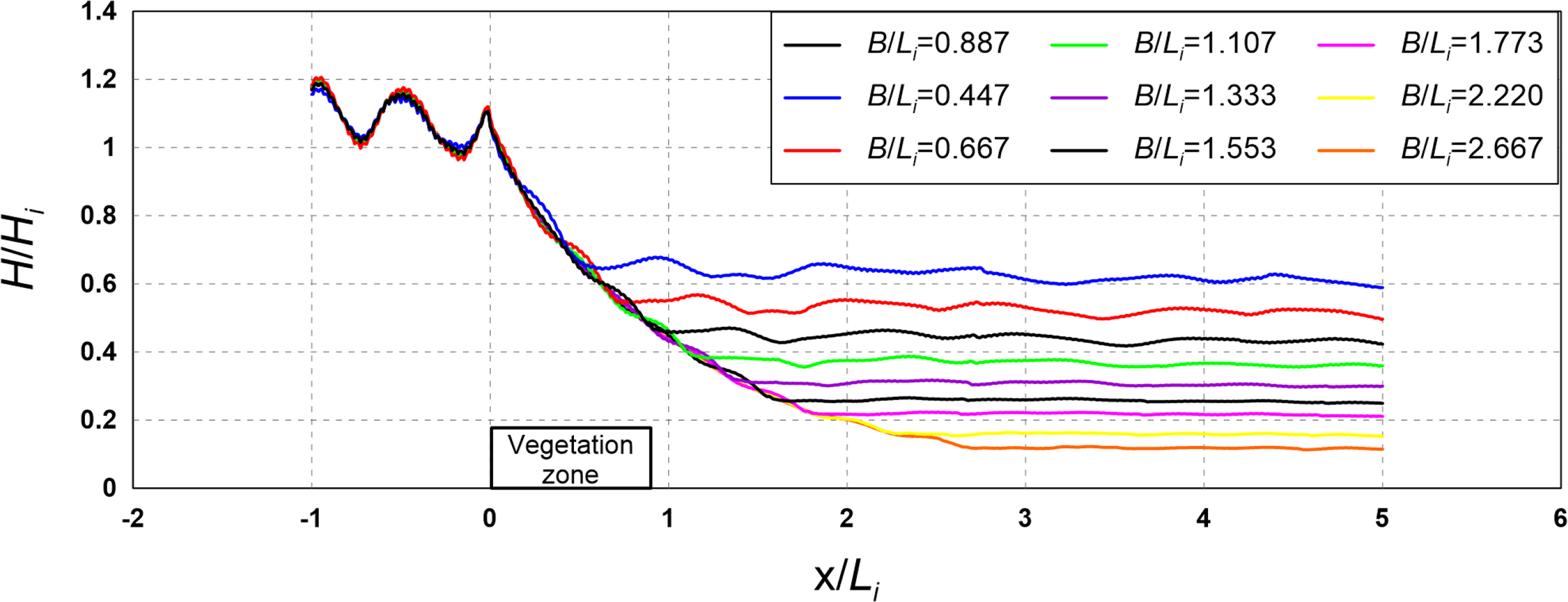
Wave height distribution according to the change in the width of the vegetation zone (B/L_i)

The abovementioned results indicate that wave attenuation increases as the width of the submerged vegetation increases, and it is judged from the flow field, vorticity distribution, and turbulence distribution that submerged vegetation is more effective for wave attenuation as energy attenuation on the crest of the vegetation increases owing to the drag of the vegetation.

4.3 Flow Field, Vorticity Distribution, Turbulence Distribution, and Wave Height Distribution According to the Density

Figs. 16 and 17 show the flow field, vorticity distribution, and turbulence distribution according to the density of the vegetation zone. Fig. 18 shows the wave height distribution around the submerged vegetation according to the density. From Figs. 16(a) and 17(a), it can be seen that the flow velocity on the vegetation crest increases as the density of the vegetation zone increases, thereby forming a strong clockwise vorticity distribution behind the submerged vegetation. From Figs. 16(b) and 17(b), it can be seen that a large turbulence distribution is formed at the crest and back of the submerged vegetation, confirming that the turbulence intensity at the back increases as the density of the vegetation increases. Therefore, the increasing wave height attenuation effect alongside the increase in the density of the submerged vegetation can be confirmed by the wave height distribution shown in Fig. 18. Additionally, from Fig. 18, wave attenuation owing to the change in the wave on the vegetation crest can be confirmed together with the increase in reflectivity as the density of the submerged vegetation increases.

Fig. 16.

Flow field, vorticity distribution, and turbulence distribution around the vegetation (Case CR-00, ρ_V = 0.123): (a) flow field and vorticity distribution; (b) flow field and turbulence distribution

Fig. 17.

Flow field, vorticity distribution, and turbulence distribution around the vegetation (Case CR-17, ρ_V = 0.213): (a) flow field and vorticity distribution; (b) flow field and turbulence distribution

Fig. 18.

Wave height distribution according to the changes in vegetation zone density (ρ_V)

The above results indicate that wave attenuation increases as the density of the submerged vegetation increases, and it is judged from the flow field, vorticity distribution, and turbulence distribution that submerged vegetation is more effective for wave attenuation as its density increases owing to the difference in energy attenuation at the crest and back of the vegetation.

4.4 Flow Field, Vorticity Distribution, Turbulence Distribution, and Wave Height Distribution According to the Arrangement Distance

Figs. 19 –21 show the flow field, vorticity distribution, and turbulence distribution according to the multi-row arrangement distance of the vegetation zone. Fig. 22 shows the wave height distribution around the submerged vegetation according to the arrangement distance. From Figs. 19(a), 20(a), and 21(a), it can be seen that the flow velocity decreases as the arrangement distance increases owing to a reduction in waves that propagate onto the vegetation crest, thereby forming a strong clockwise vorticity distribution behind the submerged vegetation. From Figs. 19(b), 20(b), and 21(b), it can be seen that a large turbulence distribution is formed at the crest and back of the submerged vegetation, confirming that similar turbulence intensity occurs despite the increase in arrangement distance. Therefore, the similar wave height attenuation effect despite the increase in arrangement distance can be confirmed by the wave height distribution shown in Fig. 22.

Fig. 19.

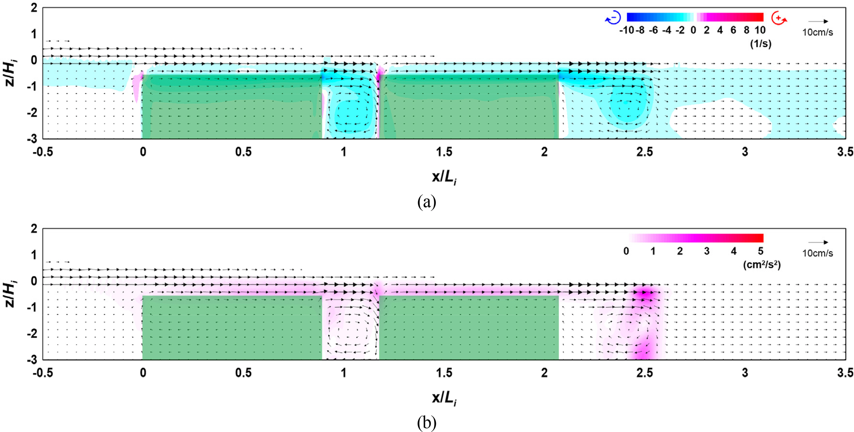
Flow field, vorticity distribution, and turbulence distribution around the vegetation (Case CR-18, V_d/L_i = 0.293): (a) flow field and vorticity distribution; (b) flow field and turbulence distribution

Fig. 20.

Flow field, vorticity distribution, and turbulence distribution around the vegetation (Case CR-19, V_d/L_i = 0.593): (a) flow field and vorticity distribution; (b) flow field and turbulence distribution

Fig. 21.

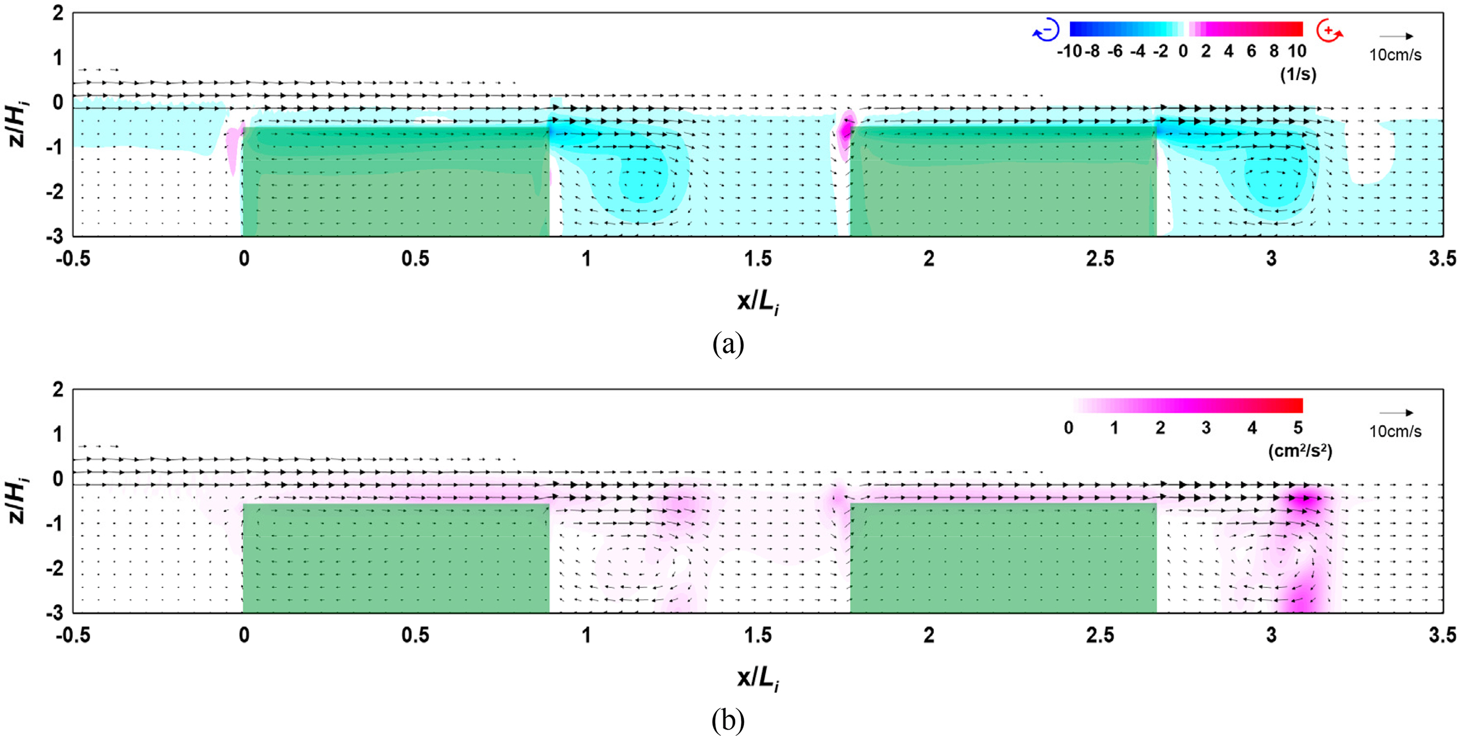
Flow field, vorticity distribution, and turbulence distribution around the vegetation (Case CR-20, V_d/L_i = 0.887); flow field and vorticity distribution; (b) flow field and turbulence distribution

Fig. 22.

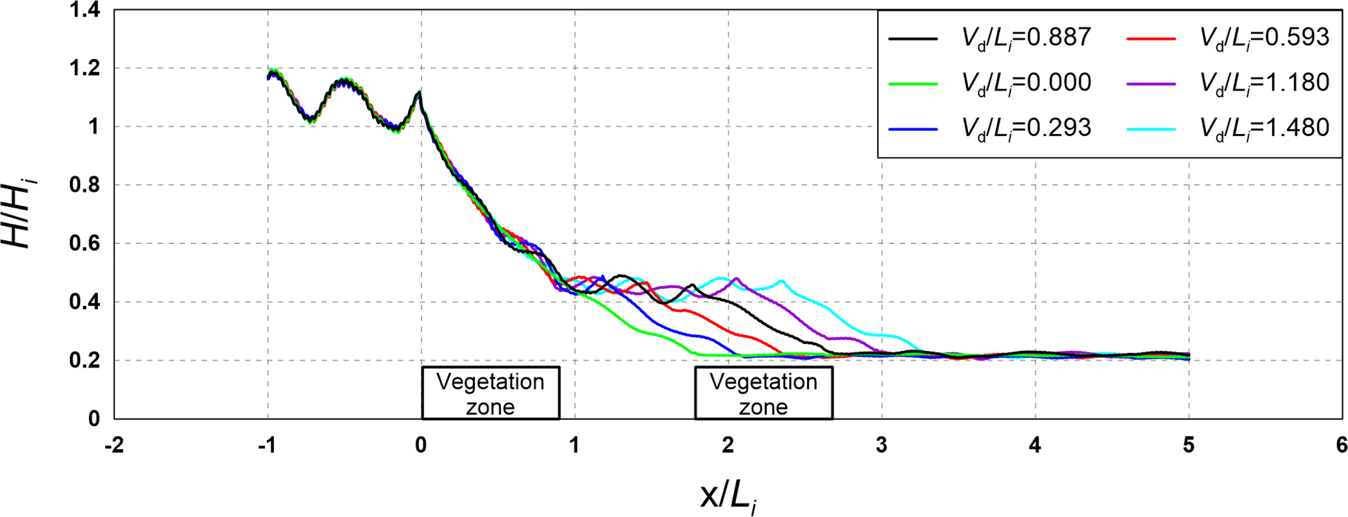
Wave height distribution according to the arrangement distance of the vegetation zone (V_d/L_i)

The abovementioned results indicate that similar wave attenuation occurs regardless of the arrangement distance. From the flow field, vorticity distribution, and turbulence distribution, we assumed that similar energy attenuation occurs owing to the drag of the submerged vegetation.

This result is contrary to the wave attenuation effect by Bragg reflection that occurs when submerged breakwaters are arranged in multiple rows. This is because the submerged vegetation has relatively low reflectivity than submerged breakwaters owing to its low porosity. However, additional examinations are required for the wave energy reduction effect according to the multi-row arrangement and arrangement distance of the submerged rigid vegetation.

5. Conclusions

A hydraulic model experiment and a numerical model experiment were performed to analyze the hydraulic characteristics according to the cross-section changes in the submerged rigid vegetation. Using the hydraulic model experiment, the reflection coefficient, transmission coefficient, and energy dissipation coefficient were analyzed according to the density, width, and multi-row arrangement distance of the vegetation zone. Using the numerical model experiment, the flow field, vorticity distribution, turbulence distribution, and wave height distribution were analyzed according to the crest depth, density, width, and multi-row arrangement distance of the vegetation zone. The following conclusions were drawn based on the results obtained.

From the hydraulic model experiment, the reflection coefficient, transmission coefficient, and energy dissipation coefficient according to the cross-section changes in vegetation were calculated. Additionally, the flow field, vorticity distribution, turbulence distribution, and wave height distribution according to the cross-section changes in vegetation were analyzed using the numerical wave tank, which was validated by comparing the results obtained from the hydraulic model experiment.
The results of the hydraulic model experiment showed that the reflection coefficient decreased as the density of the vegetation zone decreased. This is because the transmission area of waves increased in front of the vegetation zone. Additionally, we found that the transmission coefficient increased as the density and width of the vegetation zone increased. This is because more breaking waves were induced at the crest of the vegetation zone as the density and width of the vegetation zone increased.
The results of the numerical model experiment showed that the distribution and intensity of vorticity and turbulence increased at the crest and back of the vegetation zone as the crest depth of the vegetation zone decreased and width and density increased, thereby increasing the wave height attenuation performance.
When the total width of the vegetation zone was identical, the vorticity distribution, turbulence distribution, and wave height distribution according to the multi-row arrangement and arrangement distance were found to be similar. However, we believe that more examinations are required for wave energy attenuation characteristics according to the multi-row arrangement and arrangement distance of the submerged rigid vegetation.

Notes

No potential conflict of interest relevant to this article was reported.

This research was a part of the project titled “Practical Technologies for Coastal Erosion Control and Countermeasure”, funded by the Ministry of Oceans and Fisheries, Korea (20180404).

References

Abdolahpour M, Hambleton M, Ghisalberti M. 2017;The wave-driven current in coastal canopies. Journal of Geophysical Research: Oceans 122(5):3660–3674. https://doi.org/10.1002/2016JC012446 .

Anderson ME, McKee Smith J, McKay SK. 2011. Wave dissipation by vegetation. ERDC/CHL CHETN-I-82.

Asano T, Tsutsui S, Sakai T. 1988;海藻が繁茂する場の波高減衰の特性 [Wave damping characteristics due to seaweed]. Proceedings of the Japanese Conference on Coastal Engineering 35:138–142. https://doi.org/10.2208/proce1970.35.138 .

Beudin A, Kalra TS, Ganju NK, Warner JC. 2017;Development of a coupled wave-flow-vegetation interaction model. Computers & Geosciences 100:76–86. https://doi.org/10.1016/j.cageo.2016.12.010 .

Blackmar PJ, Cox DT, Wu WC. 2014;Laboratory observations and numerical simulations of wave height attenuation in heterogeneous vegetation. Journal of Waterway, Port, Coastal, and Ocean Engineering 140(1):56–65.

Cho WC. 2006;Optimum distance between multiple submerged breakwaters for wave screening performance enhancement. Journal of Ocean Engineering and Technology 20(6):82–87.

Cho YS, Lee JI, Kim YT. 2002;Hydraulic experiments on reflection of regular waves due to rectangular submerged breakwaters. Journal of Korea Water Resources Association 35(5):563–573. https://doi.org/10.3741/JKWRA.2002.35.5.563 .

Christensen ED, Deigaard R. 2001;Large eddy simulation of breaking waves. Coastal Engineering 42(1):53–86. https://doi.org/10.1016/S0378-3839(00)00049-1 .

Goda Y, Suzuki T. 1976;Estimation of incident and reflected waves in random wave experiments. Coastal Engineering Proceedings 1(15):47. https://doi.org/10.9753/icce.v15.47 .

Hadadpour S, Paul M, Oumeraci H. 2019;NNumerical investigation of wave attenuation by rigid vegetation based on a porous media approach. Journal of Coastal Research 92(SI):92–100. https://doi.org/10.2112/SI92-011.1 .

Hu Z, Suzuki T, Zitman T, Uittewaal W, Stive M. 2014;Laboratory Study on Wave Dissipation by Vegetation in Combined Current–wave flow. Coastal Engineering 88:131–142. https://doi.org/10.1016/j.coastaleng.2014.02.009 .

Hur DS, Choi DS. 2008;Effect of the slope gradient of a permeable submerged breakwater on wave field around it. Journal of Korean Society of Civil Engineers 28(2B):249–259.

Jeong YM, Hur DS. 2016;Numerical experiment of wave attenuation considering behavior of vegetation zone. Journal of Korean Society of Coastal and Ocean Engineers 28(4):232–239. https://doi.org/10.9765/KSCOE.2016.28.4.232 .

Kirby JT, Anton JP. 1990;Bragg reflection of waves by artificial bars. Coastal Engineering Proceedings 1(22)

Lee WD, Cox DT, Hur DS. 2017a;Numerical model study on the wave and current control by coastal vegetation. Journal of Coastal Research 79(10079):219–223. https://doi.org/10.2112/SI79-045.1 .

Lee WD, Park JR, Jeon HS, Hur DS. 2017b;Effects of tsunami waveform on energy dissipation of aquatic vegetation. Journal of Ocean Engineering and Technology 31(2):121–129. https://doi.org/10.5574/KSOE.2017.31.2.121 .

Manca E, Stratigaki V, Prinos P. 2010;Large scale experiments on spectral wave propagation over Posidonia oceanica seagrass. Proceedings of 6th International Symposium on Environmental Hydraulics :463–469.

Maza M, Lara JL, Losada IJ, Ondiviela B, Trinogga J, Bouma TJ. 2015;Large-scale 3-D experiments of wave and current interaction with real vegetation. Part 2: Experimental analysis. Coastal Engineering 106:73–86. https://doi.org/10.1016/j.coastaleng.2015.09.010 .

Mitsuyasu H. 1969;On the growth of wind-generated waves (II). Research Institute for Applied Mechanics, Kyushu University 17(59):235–248.

Okayasu A, Suzuki T, Matsubayashi Y. 2005;Laboratory experiment and three-dimensional large eddy simulation of wave overtopping on gentle slope seawalls. Coastal Engineering Journal 47(2–3):71–89. https://doi.org/10.1142/S0578563405001215 .

Peruzzo P, De Serio F, Defina A, Mossa M. 2018;Wave height attenuation and flow resistance due to emergent or near-emergent vegetation. Water 10(4):402. https://doi.org/10.3390/w10040402 .

Raffel M, Willert CE, Kompenhans J. 1998. Particle image velocimetry: a practical guide 2Berlin: Springer.

Raffel M, Willert CE, Wereley ST, Kompenhans J. 2007. Particle image velocimetry Berlin: Springer-Verlag. https://.org/10.1007/9783-54072308-0 .

Sakakiyama T, Kajima R. 1992;Numerical simulation of nonlinear wave interacting with permeable breakwaters. Coastal Engineering Proceedings 1(23):1517–1530.

Schumann U. 1987. Direct and large eddy simulation of turbulence. Summary of the state of art 1987 Von Karman Institute for Fluid Dynamics.

Smagorinsky J. 1963;General circulation experiments with the primitive equations: I. The basic experiment. Monthly Weather Review 91(3):99–164. https://doi.org/10.1175/1520-0493(1963)091<0099:GCEWTP>2.3.CO;2 .

van Veelen TJ, Fairchild TP, Reeve DE, Karunarathna H. 2020;Experimental study on vegetation flexibility as control parameter for wave damping and velocity structure. Coastal Engineering 157:103648. https://doi.org/10.1016/j.coastaleng.2020.103648 .

Wang H, Yin Z, Luan Y, Wang Y, Liu D. 2022;Hydrodynamic characteristics of idealized flexible vegetation under regular waves: Experimental investigations and analysis. Journal of Coastal Research 38(3):673–680. https://doi.org/10.2112/JCOASTRES-D-21-00089.1 .

Wu WC, Cox DT. 2015;Effects of wave steepness and relative water depth on wave attenuation by emergent vegetation. Estuarine, Coastal and Shelf Science 164:443–450. https://doi.org/10.1016/j.ecss.2015.08.009 .

Article information Continued

This is an open access article distributed under the terms of the creative commons attribution non-commercial license (http://creativecommons.org/licenses/by-nc/4.0) which permits unrestricted non-commercial use, distribution, and reproduction in any medium, provided the original work is properly cited.

Wave case	H_S (cm)	T_S (s)	L_S (cm)
1	2.67	0.64	60.3
2	5.33	0.64	60.3
3	2.67	0.95	107.1
4	5.33	0.95	107.1
5	2.67	1.26	150.9
6	5.33	1.26	150.9
7	9.00	1.26	150.9
8	11.00	1.26	150.9
9	2.67	1.57	193.3
10	5.33	1.57	193.3
11	9.00	1.57	193.3
12	11.00	1.57	193.3
13	2.67	1.88	234.9
14	5.33	1.88	234.9
15	9.00	1.88	234.9
16	11.00	1.88	234.9

Case	V_h (cm)	R (cm)	B (cm)	V_d (cm)	ρ_V	Number of vegetation
R1	14.8	2.2	133	-	0.123	972
R2	14.8	2.2	133	-	0.032	255
R3	14.8	2.2	266	-	0.123	1944
R4	14.8	2.2	133	133	0.123	1944

Case	Wave conditions		Vegetation zone

	H_S (cm)	T_S (s)	R (cm)	B (cm)	ρ_V
R1-01	2.67	0.64	2.2	133	0.123
R1-02	5.33	0.64	2.2	133	0.123
R1-03	2.67	0.95	2.2	133	0.123
R1-04	5.33	0.95	2.2	133	0.123
R1-05	2.67	1.26	2.2	133	0.123
R1-06	5.33	1.26	2.2	133	0.123
R1-07	9.00	1.26	2.2	133	0.123
R1-08	11.00	1.26	2.2	133	0.123
R1-09	2.67	1.57	2.2	133	0.123
R1-10	5.33	1.57	2.2	133	0.123
R1-11	9.00	1.57	2.2	133	0.123
R1-12	11.00	1.57	2.2	133	0.123
R1-13	2.67	1.88	2.2	133	0.123
R1-14	5.33	1.88	2.2	133	0.123
R1-15	9.00	1.88	2.2	133	0.123
R1-16	11.00	1.88	2.2	133	0.123
R2-06	5.33	1.26	2.2	133	0.032
R3-06	5.33	1.26	2.2	266	0.123
R4-06	5.33	1.26	2.2	133, 133	0.123

Case	Vegetation zone

	R (cm)	R/H_i	B (cm)	B/L_i	ρ_V	V_d (cm)	V_d/L_i
CR-00	2.2	0.413	133	0.887	0.123	-	-
CR-01	0.0	0.000	133	0.887	0.123	-	-
CR-02	1.0	0.188	133	0.887	0.123	-	-
CR-03	3.0	0.563	133	0.887	0.123	-	-
CR-04	4.0	0.750	133	0.887	0.123	-	-
CR-05	5.0	0.938	133	0.887	0.123	-	-
CR-06	2.2	0.413	67	0.447	0.123	-	-
CR-07	2.2	0.413	100	0.667	0.123	-	-
CR-08	2.2	0.413	166	1.107	0.123	-	-
CR-09	2.2	0.413	200	1.333	0.123	-	-
CR-10	2.2	0.413	233	1.553	0.123	-	-
CR-11	2.2	0.413	266	1.773	0.123	-	-
CR-12	2.2	0.413	333	2.220	0.123	-	-
CR-13	2.2	0.413	400	2.667	0.123	-	-
CR-14	2.2	0.413	133	0.887	0.093	-	-
CR-15	2.2	0.413	133	0.887	0.153	-	-
CR-16	2.2	0.413	133	0.887	0.183	-	-
CR-17	2.2	0.413	133	0.887	0.213	-	-
CR-18	2.2	0.413	133	0.887	0.123	44	0.293
CR-19	2.2	0.413	133	0.887	0.123	89	0.593
CR-20	2.2	0.413	133	0.887	0.123	133	0.887
CR-21	2.2	0.413	133	0.887	0.123	177	1.180
CR-22	2.2	0.413	133	0.887	0.123	222	1.480