Prediction of Wave Transmission Characteristics of Low Crested Structures Using Artificial Neural Network
Article information

Abstract
Recently around the world, coastal erosion is paying attention as a social issue. Various constructions using low-crested and submerged structures are being performed to deal with the problems. In addition, a prediction study was researched using machine learning techniques to determine the wave attenuation characteristics of low crested structure to develop prediction matrix for wave attenuation coefficient prediction matrix consisting of weights and biases for ease access of engineers. In this study, a deep neural network model was constructed to predict the wave height transmission rate of low crested structures using Tensor flow, an open source platform. The neural network model shows a reliable prediction performance and is expected to be applied to a wide range of practical application in the field of coastal engineering. As a result of predicting the wave height transmission coefficient of the low crested structure depends on various input variable combinations, the combination of 5 condition showed relatively high accuracy with a small number of input variables defined as 0.961. In terms of the time cost of the model, it is considered that the method using the combination 5 conditions can be a good alternative. As a result of predicting the wave transmission rate of the trained deep neural network model, MSE was 1.3×10⁻³, I was 0.995, SI was 0.078, and I was 0.979, which have very good prediction accuracy. It is judged that the proposed model can be used as a design tool by engineers and scientists to predict the wave transmission coefficient behind the low crested structure.
1. Introduction
As climate change causes sea levels to rise, which increases the external forces of high waves, shoreline deformation with coastal erosion and scour has received significant attention, becoming an important social issue in many countries. In particular, morphological changes in seabed due to such coastal erosion and sedimentation can cause changes in the coastal environment and ecosystems. Various deformation methods have been proposed to recover coastal erosion issues, but commercially utilized gravity-type structures such as breakwaters and headlands change the sea environment, resulting in bad seawater circulation and poor water quality. Low-crested and submerged structures (LCS), such as detached breakwater and artificial reefs, diminish the wave height with reduced wave energy behind a structure due to the change in the freeboard at the still water surface, which protects the inland sea environment. The construction of LCS is performed under specific conditions to produce the desired wave transmission coefficient; thus, the calculation or prediction of the transmission coefficient of the structure should be carried out as an important factor in designing the structure. To determine the wave transmission coefficient of LCS, various studies have proposed formulas for calculating the wave transmission rate, but the wave transmission coefficients are estimated through a regression analysis of mathematical experimental data, showing a limited analysis of the natural phenomena (Koosheh et al., 2020; Formentin et al., 2017). Recently, a machine learning model has been used to estimate and predict statistical structures from input and output data. This machine learning model can readily explain the regression analysis of nonlinear relationships (Hashemi et al., 2010; Rigos et al., 2016). Machine-learning-based prediction models employ deep learning algorithms of neural networks, which have been continuously applied in the field of coastal engineering in recent years, especially for solving problems related to modeling behavior around coastal structures (Shamshirband et al., 2020; Kim et al., 2005; Formentin et al., 2017; Panizzo and Briganti, 2007).
Herein, we introduced a prediction trend of the wave attenuation characteristics of LCS to propose an explicit method composed of weights and biases using artificial neural network. To estimate dominant factors for the wave transmission rate of LCS, we applied machine learning models to predict the wave height transmission rate of LCS dependent on 7 types of dimentionless characters with sensitivity analysis. In addition, we proposed an optimized machine learning model suitable for the determination of wave transmission coefficient and performs an overall analysis of the model with various combination. Finally, we carried out the evaluation of the applicability of the machine learning model through the analysis of the accuracy associated with the formulas for calculating the wave height transmission rate of the existing LCS. We found that the estimated wave attenuation characteristics calculated with the presented weight and bias matrix shows better accurate reliability compared with those obtained from the broadly used empirical formula.
2. Background
2.1 Analysis of Transmission Coefficient Empirical Formulas
Among various studies, Takayama et al.(1985) proposed the Eq. (1) to determine the wave transmission coefficient for LCS based on empirical experiment using irregular wave as follows:
Goda and Ahrens (2009) proposed the formula of wave transmission coefficient for LCS as follows.
Herein, Beffis effective crest width at still water level, Bswl is the width of structure at still water level, B is the crest width of structure, B0is the width at the bottom of structure.
Calabrese et al. (2003) used the large-scale experimental data to determine the wave transmission coefficient.
2.2 Artificial Neural Network
Artificial neural network (ANN) is modeling systems that provides a data process structure inspired by the neural networks of human brains, which are composed of a web of millions of interconnected neurons. A neuron is a special biological cell that conveys information from one neuron to others. ANN is composed of a large number of simple processing elements interconnected with each other. The system requires the involvement of a labeled direct graph structure where nodes conduct computations. The “directed graph” provides a set of “nodes” (vertices) and a set of “connections” (edges/links/arcs) to connect pairs of nodes. In a neural network, each node performs simple computations, and each connection delivers a signal from one node to another, labeled by a number called the “connection strength” or “weight”, which implies the extent to which a signal is amplified or diminished by connection, as shown in Fig. 1.
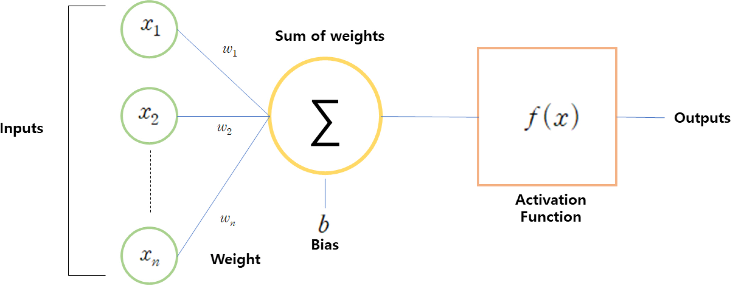
Neural network diagram of element
In the ANN data process, the result values are derived by substituting the normalized input variable into the function of Eq. (13) at each node.
2.2.1 Activation function
The activation function provides the explanation of non-linearity by substituting the estimated input data in each node into a function that creates non-linearity and then outputs the results. Different kinds of functions, such as linear, exponential, sigmoid, tanh, rectified linear unit (ReLU), softmax, scaled exponential linear unit (SeLU), and expoenetial linear unit (elU) are utilized for the activation function. The mean squared error of the various functions where six different activation functions are described to the hidden layer and output layer as shown in Fig. 2.

Type of activation functions: (a) Sigmoid type; (b) Tanh type; (c) ReLU type; (d) Exponential type; (e) eLU type; (f) Softmax type
2.2.2 Gradient decent method
In general, the error back propagation method is used as an optimization algorithm for parameter estimation, which re-updates any parameter to the one with the lowest error. The period in which each parameter is updated once is called the weight adjustment period (epoch). Here, the error backpropagation refers to the process of minimizing the error by re-correcting the weight while going backwards the result of the sum of the errors of each neuron. For the optimization of the loss function, the gradient descent method was developed by re-updating the weights to find the lowest point of the lost value. The existing gradient descent method can accurately derive weights, but it has a disadvantage in that the amount of calculation is very large because it must be differentiated over the entire data instantaneously whenever the weights are changed. That is, the speed may decrease due to the load caused by a large amount of computation, and learning may be stopped before additionally finding the optimal solution. To compensate for this problem, various advanced gradient descent techniques have been developed. Advanced gradient descent techniques include stochastic gradient descent (SGD), momentum, Nesterov accelerated gradient, Adagrad, and root mean square propagation (RMSProp), Adam, etc., and in this study, the optimization process using Adam was performed. Adam is a gradient descent method that combines Momentum and RMSprop techniques, and uses the exponential average of the squares of the slopes of the RMSprop technique. is as follows (Eqs. (14)–(16)).
-
Stochastic gradient descent (SGD)
The stochastic gradient descent method consists of a set of parameters to be updated through the calculation of the change rate of the loss function (E) and the learning rate (η) shown in Eq. (14).
(14)Here, W is a weight, η is a learning rate, E is an error, and is a method of updating weights according to a constant learning rate (η) using some randomly extracted data.
-
Adaptive gradient, Adagrad
In the adaptive gradient method, the learning rate is adjusted according to the number of updates of the variable by ht when the weights are re-updated, and the weights are trained to reach the optimal value. It is a method of learning by decreasing the learning rate for variables that have changed significantly and increasing the learning rate for variables with small changes (Eqs. (15), (16)).
(15)(16)Here, for weight update, the learning rate is multiplied by
-
RMSprop
In the complex structure of Adagrad, there is a problem that the learning rate becomes 0 before reaching the global minimum. To compensate for this, the RMSprop technique was developed (Eqs. (17), (18)). This method improved the existing problems by reflecting and accumulating the latest slope information using the Decaying mean.
(17)(18)Here, ρ is added to the ht parameter, which usually uses a value of 0.9 as the attenuation rate, and functions to reflect the latest gradient information rather than simply accumulating the weight gradient.
-
AdaDelta (Adaptive delta)
AdaDelta is calculated using the Hessian matrix instead of the learning rate to compensate for the problem of small learning rate in Adagrad, and is calculated as follows Eqs. (19)–(22).
(19)(20)(21)(22) -
Adam (Adaptive moments)
Adam uses the exponential averaging of the square of the slope of the RMSprop technique as a gradient descent method that combines the Momentum and RMSprop techniques (Eqs. (23)–(25)).
(23)(24)(25)Here, mt is the estimate for the first moment of the gradient, vt is the estimate for the second moment, and β1 and β2 are the correction values that correct the deviation of the weights.
3. Methodology
3.1 Experimental Database
It is required to consider various valuables to determine the wave transmission characteristics behind the LCS structure. The optimal machine learning model was used to figure out the role of variables affecting the wave control of LCS using the machine learning analysis package. We used the results of previous hydraulic experiment with LCS for input data, including deep sea wave length (L0), crest freeboard (RC ), incident wave height (H0), crown width (B), water depth (h), structure height (hc), wave period (T0), similarity coefficient for breakwater (tanα) and Dn50(Seelig, 1980; Daemrich and kahle, 1985; van der Meer, 1988; Daemen, 1991) (Table 1). Data was obtained from DELOS databased of submerged breakwater information.
- 81 data on rubble mound emerged/submerged breakwater [Seelig];
- 95 data on tetrapod submerged breakwater [Daemrich and Kahle];
- 31 data on rubble mound emerged/submerged breakwater [Van der Meer];
- 53 data on rubble mound emerged/submerged breakwater [Daemen]

Ranges of parameter of reference
When applying the results of the mathematical model experiment, applying a dimensionless factor helps to clarify the problem related to the scale effect. Therefore, we applied 7 dimensionless factors as input variables as shown in Table 2 in consideration of the above dimension factors.

Definitions and ranges of scaled model parameter
3.2 Hyperparameters Tuning and Model Validation
A machine learning model has many hyperparameters that the user needs to specify. It is used to optimize performance by balancing bias and variance of machine learning models. Random search cross-validation (CV) and grid search CV are methods for deriving hyperparameters suitable for models and data. In this study, the optimal parameters for predicting the wave height attenuation characteristics of low-rise structures were derived using grid search CV. Table 3 shows the parameters and ranges applied to the grid search CV, and the parameter with the highest accuracy was derived through the calculation of a total of 960 cases.
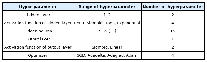
Hyperparameter tuning
The purpose of a machine learning model is to predict with high accuracy on new data, and to ensure generalization and reliability of model performance on new data. Cross-validation is a method to improve the generalization performance of a model and is generally a more reliable and superior statistical evaluation method than dividing the training set and test set once. The most widely used cross-validation method is k-cross-validation, which was developed to minimize the bias associated with random sampling of the training set. In this study, 10-fold cross validation was performed, the entire data sample was divided into 10, 9 were used for training and 1 was used for model validation, and cross-validation was performed 10 times in a row (Fig. 3).
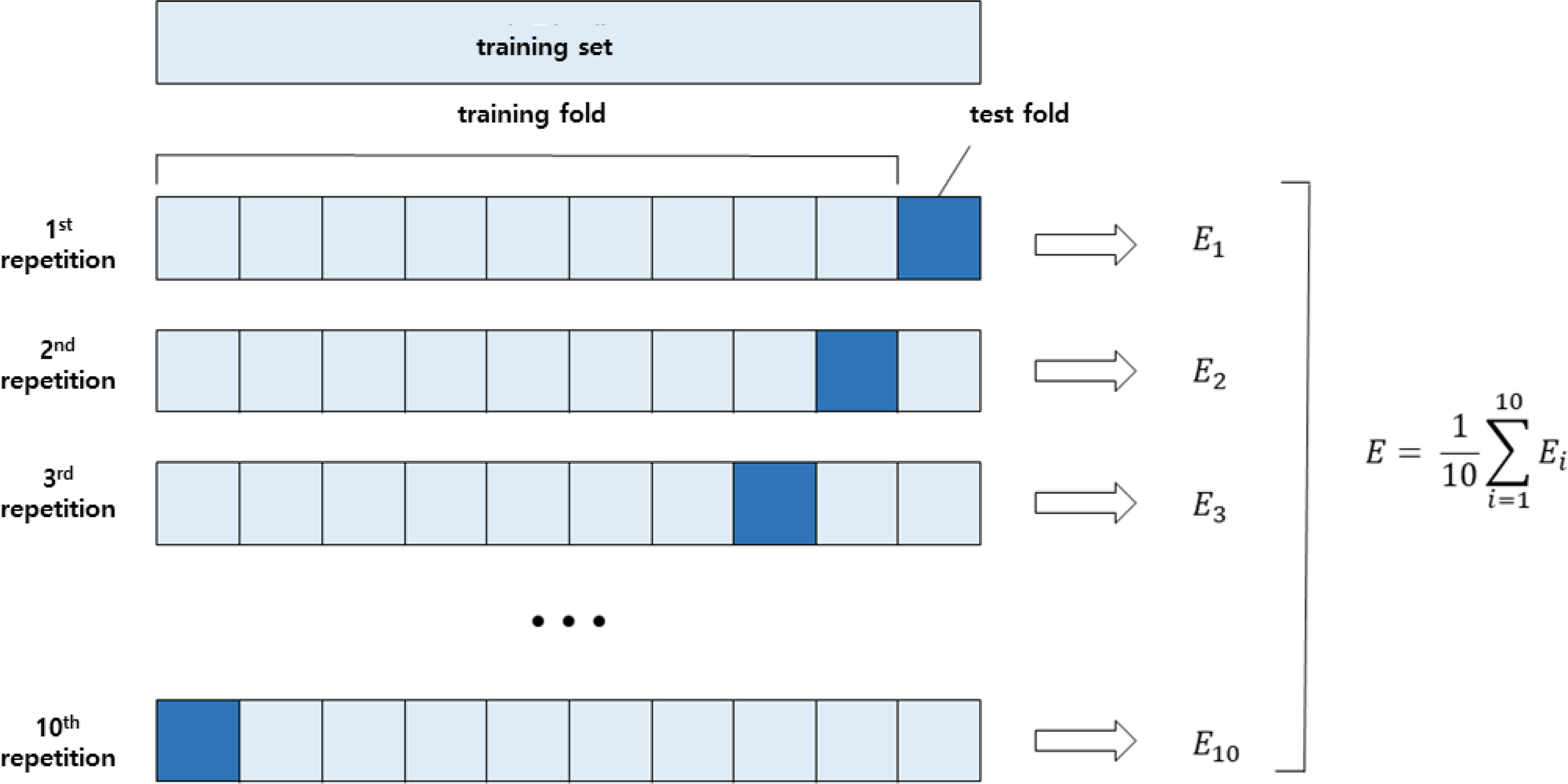
10-fold cross validation
3.3 ANN Model Setup
Table 4 shows ANN model setup. In this study, we utilized the 260 sets of wave input data with reference to the results of the hydraulic model experiment with existing low crest structures. Of the total 260 data, we used 70% as training data and 30% as prediction data. To set up the prediction model of wave properties with high accuracy using LCS method, various hyperparameters were determined under different conditions, including the activation function, gradient descent technique, hidden layer, and overfitting prevention technique, to build a model with low error and high accuracy. With respect to the activation functions of the hidden layer and the output layer, optimal activation functions (ReLU, Sigmoid) were applied using various model prediction results. We applied the calculated value to the hidden layer’s activation function (ReLU) to explain non-linearity. We calculated the result by substituting the hidden layer calculation result into the function of output layers and output the result value by inputting it into the activation function (Sigmoid) of the output layer. To verify the model performance, we applied 10-fold cross-validation method that was developed to minimize the bias associated with random sampling of the training set.
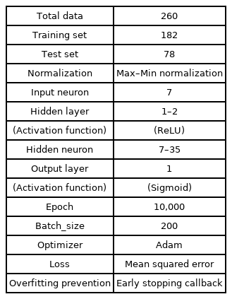
Model setup of ANN model
The neural network derives an optimal weight and bias where the mean squared error (MSE) is minimized through the error backpropagation method. In the process of weight redistribution using backpropagation algorithm, the increase in the number of hidden layers and hidden nodes improves the model’s performance, but increases training costs. Thus, this study determined various hyperparameters with respect to the number of hidden layers and hidden neurons. We analyzed model accuracy (R2) under the condition of the 1st–3th layers and 7–35 hidden neurons at hyperparameters.
When building a neural network, the optimal training time and prediction performance are obtained by varying the number of hidden layers and neurons. Fig. 4 reveals the R2results for the training set and the test set for the hidden neuron under the condition of different hidden layers, which shows trend lines with R2 values with respect to the number of hidden layers and hidden neurons for training data. It represents that the model accuracy increases with the increase in the numbers of hidden layers. In addition, R2value of the training set gradually increases as the number of hidden neurons increases. On the other hand, the model accuracy of the test set increases as the number of hidden layers increases under certain condition (Fig. 5). The R2 value (0.979) of the test set showed the highest accuracy under the condition of 29 hidden neurons with 2 hidden layers, which suggests that the model accuracy of the test set does have a high relationship with the accuracy of training set under certain condition. Thus, we constructed the model under the optimum condition of 29 hidden neurons with 2 hidden layers.
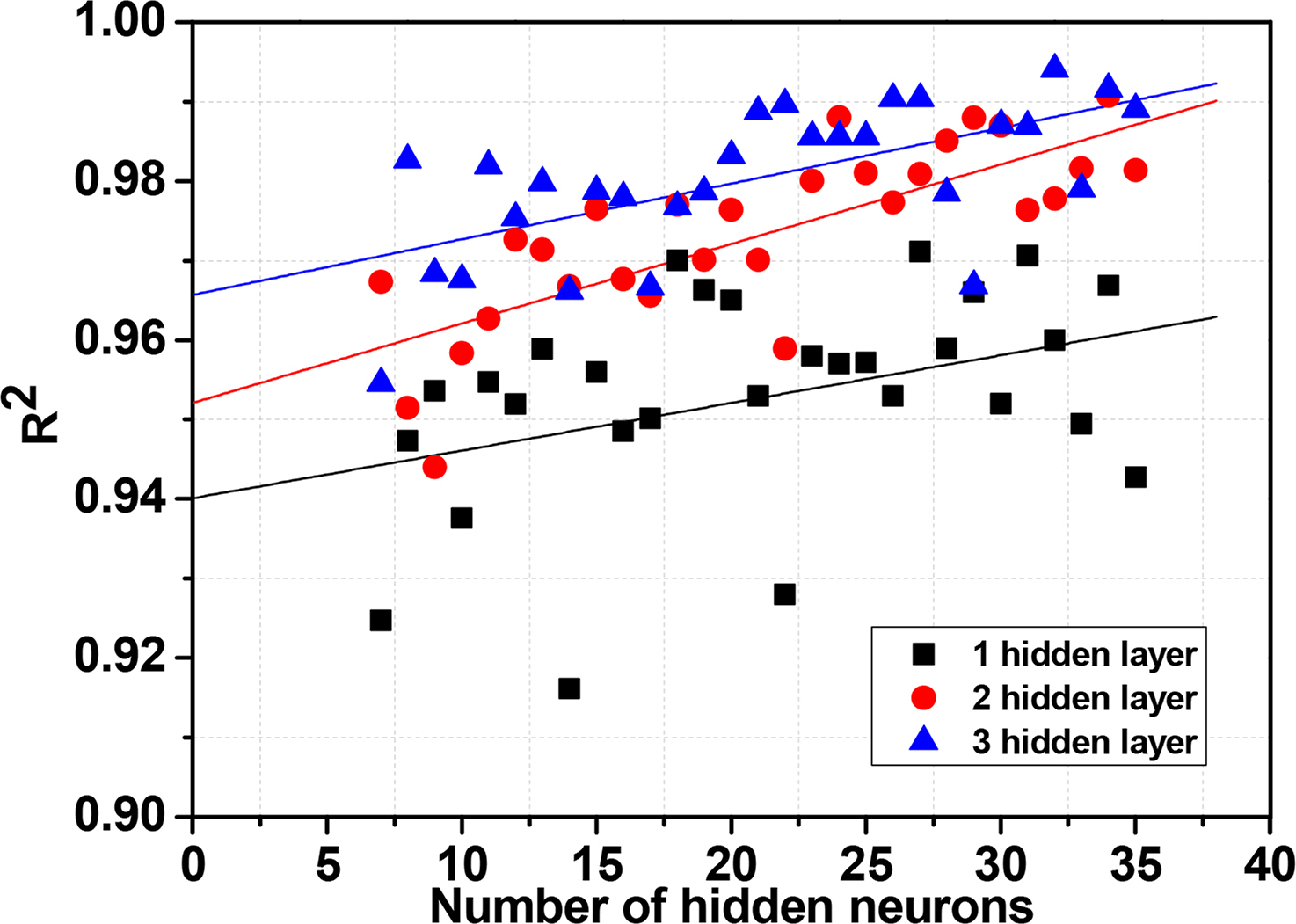
R_squared of training data as a function of the number of hidden layer
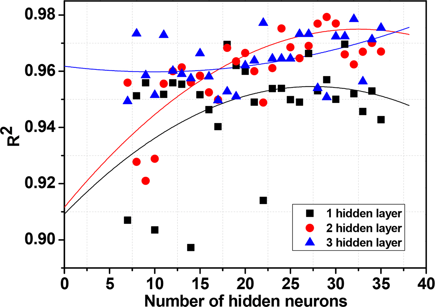
R_squared of test data as a function of the number of hidden layer
4. Results and Discussion
4.1 Estimation of Wave Transmission Rate Using Empirical Formula
As shown in Fig. 6, we compared the experimental values of wave transmission rate with those obtained from empirical formula. Takayama et al. (1985) suggested an estimated wave transmission rate that has an MSE of 0.021 and an R 2 value of 0.5, which reveals the overestimation of experimental results with a low accuracy (Fig. 6(a)). Some data even broke the pattern of effective wave transmission rate (0 < Kt < 1), driven by the case of high relative freeboard. Takayama’s formula can mainly use for the submerged structure under still water level, and the empirical formula are composed of the linear regression type of the 1st order of polynomial equation, which cause the low accuracy.
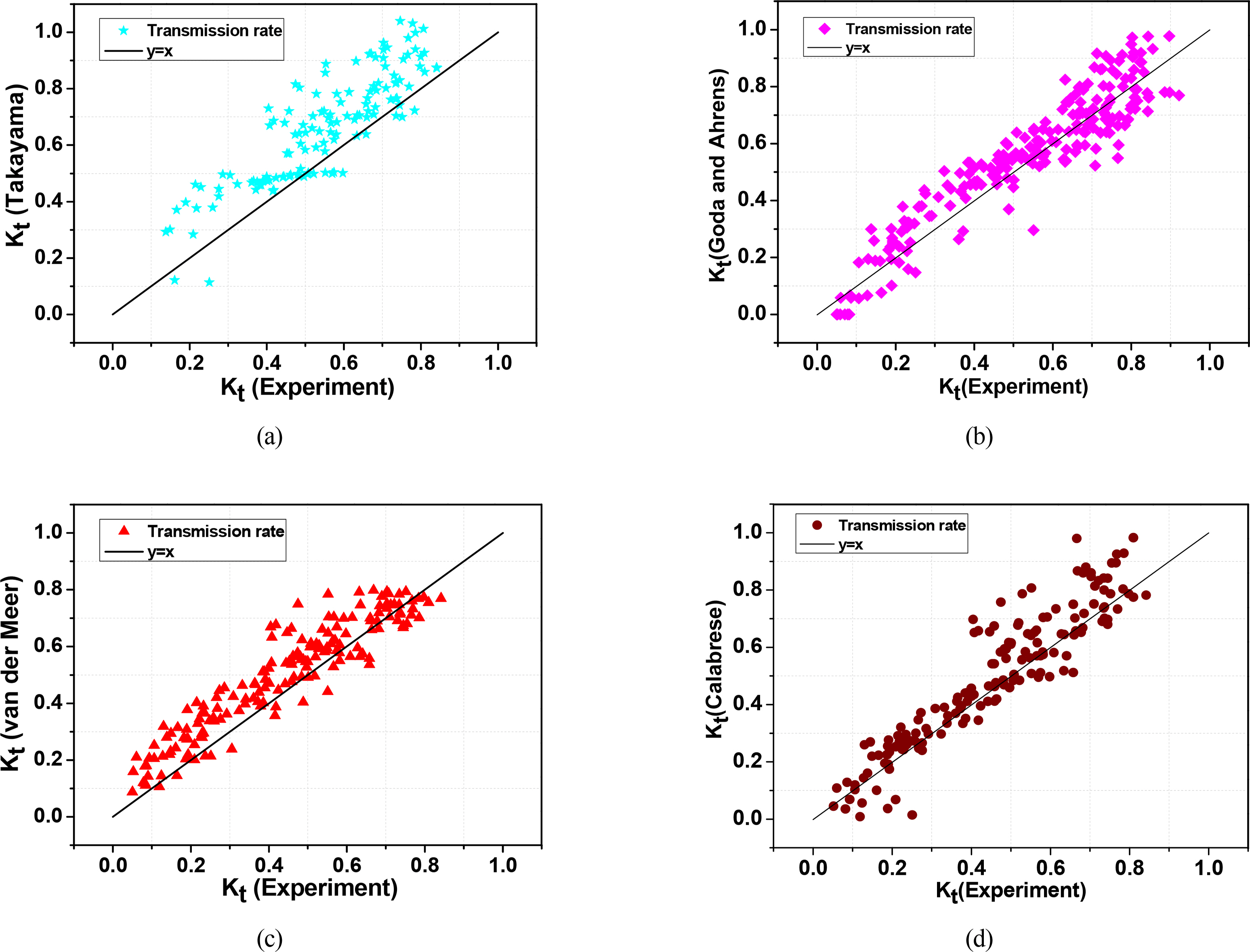
Comparison of wave transmission formulas with experimental data: (a) Takayama et al. (1985); (b) Goda and Arhens. (2008); (c) Van der Meer et al. (2005); (d) Calabrese et al. (2003)
Among four different empirical formulas, Goda and Ahrens (2008) revealed the estimated wave transmission rate that has an MSE of 0.008 and an R 2 value of 0.851, which shows the highest accuracy because suggested formula used 6 types of dimensionless numbers for converted effective crest width (Beff) under various conditions (Fig. 6(b)). Fig. 6(c) shows the estimated wave transmission rate of LCS suggested by Van der Meer et al. (2005). The effective values of wave transmission rate are obtained in the range of 0.075 < Kt < 0.8 in the empirical formula. They provided an MSE of 0.009 and an R 2 value of 0.81, which generally represent overestimated results compared to experimental results. In the same manner, the results, obtained from Carabrese et al. (2003) provides the overestimated prediction at the point of wave transmission rate compared to the experimental results, as shown in Fig. 6(d), suggesting inappropriate model for our study.
4.2 Prediction Accuracy Analysis Using ANN
Figs. 7 and 8 show the wave transmission rate of the training and test data of 206 sets using a deep neural network under the optimum condition of 29 hidden neurons with 2 hidden layers. In the figures, the horizontal axis reveals the experimental values, and the vertical axis shows the distribution of predicted values. In the prediction results of the training dataset, index of agreement (I) was 0.997, scatter index (SI) was 0.086, and R2 was 0.988. For the test dataset, MSE was 1.3×10⁻³, I was 0.995, SI was 0.078, and R2 was 0.979, suggesting that the predictive model for the wave transmission rate demonstrated excellent performance. Based on the obtained analysis, it is worth noting that the performance prediction method using an artificial neural network model can be suitable for various fields in coastal engineering, unlike the broadly used empirical formula. Table 5 shows the statistical model performance results based on the application of popular empirical formula compared to deep neural network, which suggests that the ANN model provides a more accurate prediction performance compared to the empirical formula. In addition, the ANN model is not required to set up the effective range of the wave transmission rate or apply the special formula dependent on the input variables whereas the empirical formula can be used under the recommended effective range in order to diminish the uncertainty. Thus, the ANN model can provide high prediction accuracy with cost-effective reliability when only seven dimensionless input variables are used.
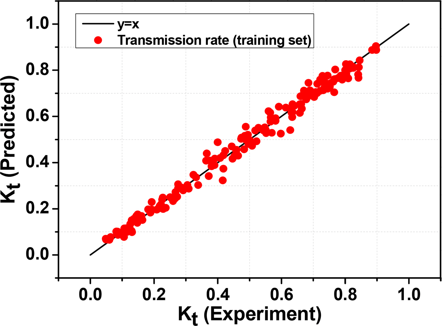
Comparison of transmission rate between experiment and prediction (training data)
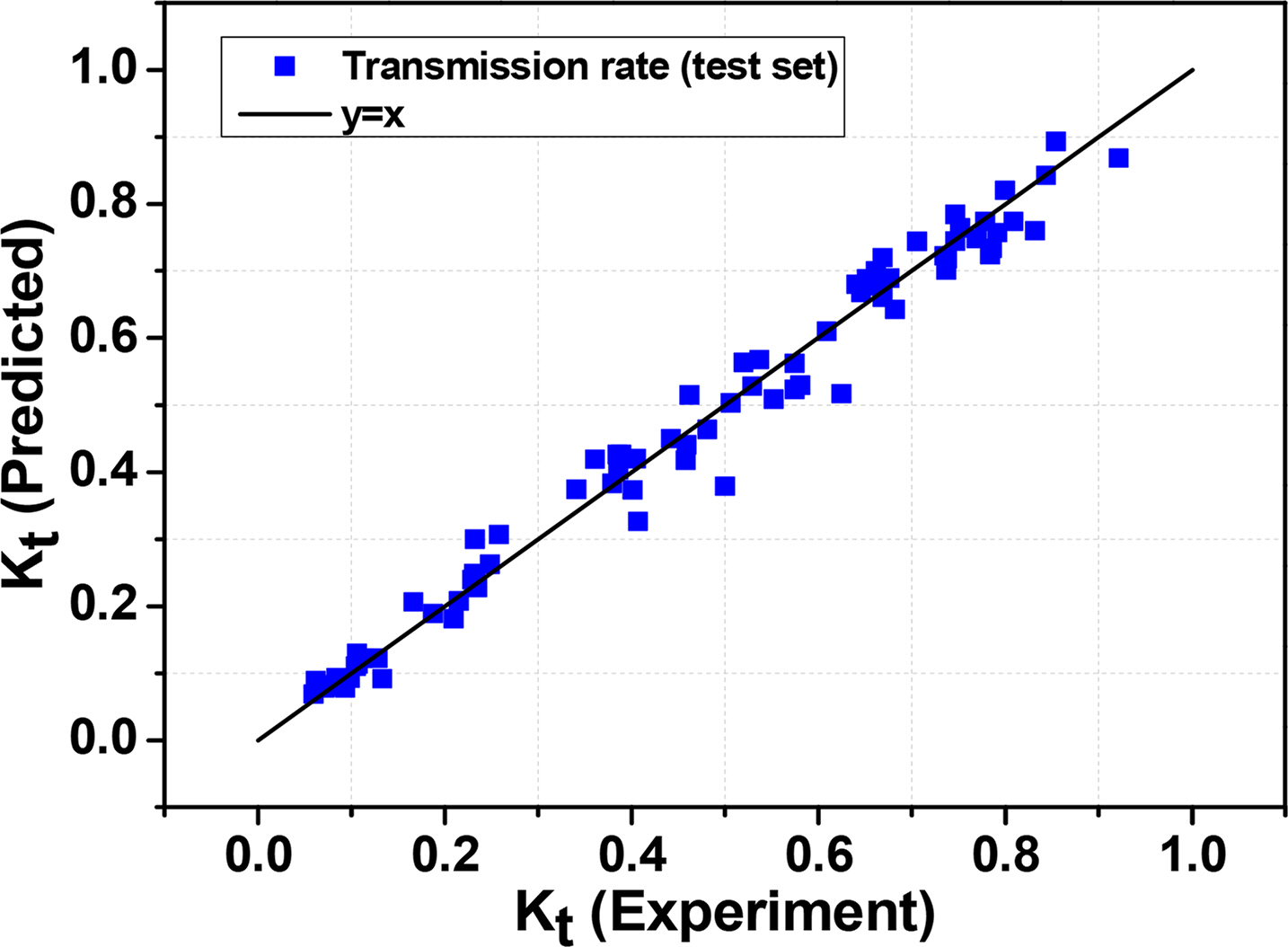
Comparison of transmission rate between experiment and prediction (test data)

Statistical parameters of the results
4.3 Sensitivity Analysis
To estimate the independent importance of the input variable of the model constructed using ANN calculations and to determine the important input variables, we performed a sensitivity analysis of the effect on the prediction of the wave transmission rate through model application using the same training set. Table 6 shows the sensitivity analysis results of the wave transmission rate for each input variable. To estimate the independent importance of the input variable of the model constructed using ANN calculations and to determine the important input variables, we performed sensitivity analysis of the effect on the prediction of the wave transmission rate through model application using the same training set. The analysis reveals that the model accuracy for the relative freeboard (RC/H0) had an MSE of 146.7×10⁻³ and an R2 value of 0.153, which was found to be the most important parameter for the wave attenuation and wave transmission rate of the structure. This finding is attributed to the reduction of transmitted wave height along with strong breaking wave, and an increased reflected wave in front of the structure as the crown depth is reduced. Figs. 9 (a) and (d) are the distributions of the experimental and predicted values, respectively, when factors related to the relative freeboard and ratio of the crest height to the water depth are excluded, which showed that the predicted value using the model overestimated the experimental value and the error increased significantly. As the relative freeboard factor is the dominant factor in wave control, a large error occurred when the two factors were not considered.
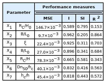
Sensitivity analysis of ANN model
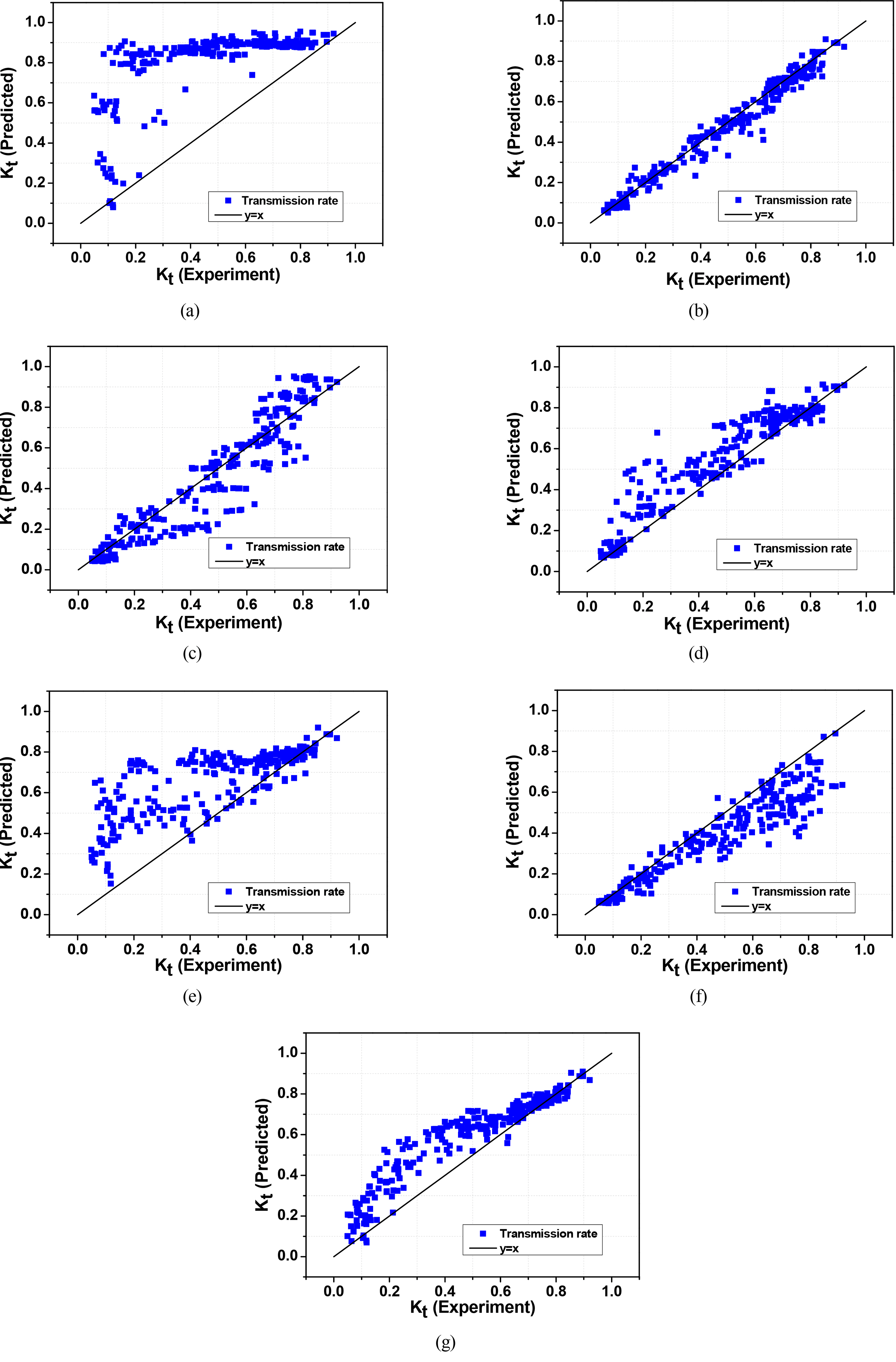
Sensitivity analysis of input variables: (a) RC/H0 variables of sensitivity; (b) B/H0 variables of sensitivity; (c) ξ variables of sensitivity; (d) B/L0 variables of sensitivity; (e) RC/h variables of sensitivity; (f) Dn50/hc variables of sensitivity; (g) hc/h variables of sensitivity
Most of empirical formular(van der Meer, 2005; Goda, 2008; Calabrese, 2003; Takayama, 1985) have suggested r elative freeboard (RC/H0), ratio of the crest width to wave length (B/L0) and surf similarity parameter (ξ) as impact factors for wave attenuation coefficient. However, sensitivity to the wave breaking similarity coefficient reflecting the conditions for the front slope and wave slope of the structure was MSE 22.4×10⁻³, R 2 0.703, which was less sensitive to wave control than other variables. The standard deviation of the input variable is large, and the interpretation of various conditions of the crest width to wave length is insufficient because wave transmission rate was performed for two widths of 0.3 and 1.0, in the input variable. In all experiments and model implementation, the variable control is considered one of the important factors for obtaining reliable results. Therefore, in future research, we plan to develop a model with high predictive performance through the development of various machine learning-based predictive models using refined input variables.
4.4 Analysis of Accuracy Metric According to Input Variables Combination
In this study, we applied input variables composed of seven dimensionless numbers (X ={

Influence of number of input; variables: (a) Combination 1; (b) Combination 2; (c) Combination 3; (d) Combination 4; (f) Combination 6; (g) Combination 7; (h) Combination 8
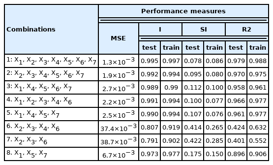
Performance measures for analysis of different input variable combinations
Combination 7, applying three input variables (
Furthermore, accurate prediction using neural network model requires reducing training time and improving the simplicity of the model. An ideal model is one that describes the problem in the easiest and simplest way using the fewest variables. Therefore, it is important to identify variables that save modeling time and space.
Accordingly, combination 4 using four input variables produced a result with relatively high accuracy, with an MSE of 2.5×10⁻³ and R 2 of 0.961. In terms of the model time cost, combination 4 offers a good alternative for the model.
4. Conclusion
In this study, we built a deep neural network model to predict the wave transmission rate of low crested structures using TensorFLow, an open source platform. To construct the model, we utilized the hydraulic model experiment data from Seelig (1980), Daemrich and kahle (1985), van der Meer (1988), Daemen (1991) for training (70%) and prediction (30%). These neural network models show reliable prediction performance and are expected to be widely used in practical applications in the field of coastal engineering.
The sensitivity analysis using the neural network model found that importance of independent variable input for relative freeboard (RC/H0) and ratio of the crest height to the water depth (RC/h) was large, and the lowest performance appeared when the two factors were excluded from training. In short, the crest depth was found to be the most dominant factor influencing the wave height attenuation in the hydraulic behavior around the low crested structure.
The proposed model showed relatively high accuracy in predicting the wave transmission coefficient of the low crested structure according to various combinations of input variables, with combination 5 showing 0.961 despite using a small number of input variables. In terms of the model time cost, a method using combination 5 offers a good alternative.
The prediction results were analyzed using a comparative review of the results from the existing empirical formula and statistical indicators. The result of wave transmission rate of the trained deep neural network model showed very good prediction accuracy, with 1.3×10⁻³ of MSE, 0.995 of I, 0.078 of SI, and 0.979 of R 2, the prediction performance is highly improved compared to existing empirical results. Engineers and scientists can use the suggested model as a design tool to predict the wave transmission coefficient behind the low crested structure.
Notes
Soonchul Kwon serve as an editor of the Journal of Ocean Engineering and Technology but has no role in the decision to publish this article. No potential conflict of interest relevant to this article was reported.
This work was supported by a 2-Year Research Grand of Pusan National University.