Proposal of Parameter Range that Offered Optimal Performance in the Coastal Morphodynamic Model (XBeach) Through GLUE
Article information

Abstract
The process-based XBeach model has numerous empirical parameters because of insufficient understanding of hydrodynamics and sediment transport on the nearshore; hence, it is necessary to calibrate parameters to apply to various study areas and wave conditions. Therefore, the calibration process of parameters is essential for the improvement of model performance. Generally, the trial-and-error method is widely used; however, this method is passive and limited to various and comprehensive parameter ranges. In this study, the Generalized Likelihood Uncertainty Estimation (GLUE) method was used to estimate the optimal range of three parameters (gamma, facua, and gamma2) using morphological field data collected in Maengbang beach during the four typhoons that struck from September to October 2019. The model performance and optimal range of empirical parameters were evaluated using Brier Skill Score (BSS) along with the baseline profiles, sensitivity, and likelihood density analysis of BSS in the GLUE tools. Accordingly, the optimal parameter combinations were derived when facua was less than 0.15 and simulated well the shifting shape, from crescentic sand bar to alongshore uniform sand bars in the surf zone of Maengbang beach after storm impact. However, the erosion and accretion patterns nearby in the surf zone and shoreline remain challenges in the XBeach model.
1. Introduction
Morphological changes in nearshore areas result from complex, nonlinear processes variable by the interaction of waves, sediment transport, ocean current, and water depth. Additionally, coastal phenomena of various scales occur because of spatiotemporal variability, making it difficult to accurately identify the behavior of various morphological changes in nearshore areas up until now. Because of these complex nearshore processes, modeling morphological changes involves uncertainties caused by boundary conditions, input data, model calculation equations, and parameters (Baquerizo and Losada, 2008). Thus, quantitative evaluation toward predicting uncertainties is essential for accurate numerical modeling of morphological changes in nearshore areas.
XBeach (Roelvink et al., 2009), an open-source numerical model for morphological changes in nearshore areas developed by Deltares in the Netherlands, is widely used because it can simulate morphological changes by combining with various fluid dynamic and morphodynamic processes based on physical phenomena. However, the XBeach model was initially developed to simulate a collapse in a barrier island located on the coast of the States of Louisiana and Texas because of Hurricane Katrina. Previous studies have indicated the issue of erosion induced by excessive prediction of sand movement in the open sea direction under storm conditions where the default settings of the parameters are typical (Do et al., 2018; Elsayed and Oumeraci, 2017; McCall et al., 2010). Furthermore, parameterization processes are included to represent nonlinear processes not yet completely identified, which essentially requires the calibration of parameters to enhance the model’s accuracy under various sea and wave conditions. For the calibration of parameters in XBeach, the use of a new empirical constant setting based on experimental and field data (Do et al., 2018; Jin et al., 2021), the proposal of a new empirical formula, and the introduction of parameters based on physical phenomena (De Vet, 2014; Elsayed and Oumeraci, 2017; McCall et al., 2010) have been attempted. However, the trial-and-error method has been widely used as a typical calibration method. Thus, the trial-and-error method is a passive calibration method performed on the basis of the research experience and knowledge of model users, and it is difficult to comprehensively consider a range of parameters. As such, a combination of parameters proposed by the trial-and-error method cannot be applied if it is out of the target sea area It also connotes the risk of the user’s subjectivity being inherent (Ruessink, 2006; Simmons et al., 2017). To overcome this obstacle, Simmons et al. (2017) combined XBeach with the generalized likelihood uncertainty estimation (GLUE), which has been used in other research fields for systematic calibration and parametric objectivity, to conduct a study on estimating new parameters and assessing uncertainties.
The GLUE technique is known as a systematic parameter calibration method that can remedy the drawback that the user’s subjectivity could be inherent when selecting parameters through trial-and-error. The basic premise is that GLUE is performed on the basis of equifinality, which can derive the same level of prediction performance at the various input conditions caused by nonlinear interaction and uncertainties when modeling is conducted to reproduce a specific phenomenon (Beven, 2006). Afterward, a combination of numerous parameters created by Monte Carlo sampling is numerically simulated, thereby selecting the optimal combination of the parameters based on the likelihood calculated by quantifying the accuracy of the simulated results and removing various uncertainties. Simmons et al. (2017) applied the GLUE technique to Lido Di Classe in Italy as a study sea, in which the calibration of XBeach had already been conducted using a trial-and-error method by Harley et al. (2016), to select the optimal combination of parameters and compared their result with that of Harley et al. (2016). Thus, they discovered that GLUE required more numerical simulation cases and took more time to calculate than the trial-and-error method did, but the prediction performance was successfully improved by objectively considering a wide range of parameters. They also suggested the changing sensitivity of XBeach parameters according to the nearshore morphological change (overwash or collision regime) via the storm effect defined by Sallenger (2000) using the GLUE technique. Simmons et al. (2019) selected three nearby beaches, including Narrabeen beach in Sydney, Australia, as a study area and quantified and calibrated the one-dimensional (1D) simulation results through GLUE. In doing so, they successfully simulated beach erosion after a storm in Narrabeen, and XBeach showed a significant improvement in prediction performance when calibrating parameters using one or more storm event datasets, suggesting the importance of calibration for numerical simulation. They also generalized the optimal parameters of the three beaches through GLUE and proposed different parameter values for each beach, reported as an effect of beach characteristics.
As described above, previous studies demonstrated successful one-dimensional (1D) numerical simulation results when applying GLUE to XBeach. However, for regions where morphological changes in the alongshore direction are prominent, such as the eastern coast of Korea, where a crescentic sand bar was developed, it is essential to have a numerical simulation incorporating two-dimensional (2D) coastal processes, such as cross-shore sediment transport along with alongshore sediment transport and sediment transport by a nearshore current. Thus, this study verified the applicability of GLUE to 2D XBeach simulation results, not studied much until now, proposed an optimal range of parameters, and analyzed uncertainties.
2. Study Methodology and Field Data Analysis
2.1 Introduction of the XBeach Model and GLUE
XBeach has been widely used to simulate hydraulic characteristics and the morphodynamic response of nearshore areas, such as dunes and sandy beaches, during storms in various coastal engineering fields. XBeach is a 2D numerical model that calculates wave propagation and morphological changes by combining fluid dynamics and morphodynamic processes on the basis of physical phenomena under short-term storm wave conditions. Particularly, it has the advantage of simulating infragravity waves using a nonlinear shallow water equation under the surf-beat mode. However, nonlinear processes are characterized by inherent numerous free parameters because of inadequate understanding of breaking waves, sediment transport, etc., which are represented through parameterization in XBeach (Bolle et al., 2010; McCall et al., 2010; Roelvink et al., 2009). It also has a limitation in that the default parameter setting in the model excessively assesses sediment transport in the open sea direction and induces excessive erosion under general storm conditions because it was designed to simulate a barrier island collapse caused by Hurricane Katrina at the time of the development. To overcome this roadblock, calibration of parameters is essentially required, and several studies have been conducted on calibration.
Generally, XBeach is calibrated through a passive trial-and-error method considering only partial parameters based on the researcher’s experience and prior studies. However, this study employed GLUE as a new parameter calibration technique. GLUE is a departure from a passive calibration method that considers only a single parameter one at a time, as is done in a trial-and-error method, but instead selects a range of parameters when conducting a calibration to produce many combinations through Monte Carlo sampling. Thereby, it takes recourse to an active calibration method to conduct numerical simulations and quantification systematically and sequentially. As GLUE conducts numerical simulations of many combinations, it relatively takes a great deal of simulation time, but it has the advantage of increasing the reliability of the final proposed parameters and quantitatively analyzing uncertainties inherent to numerical models.
2.2 Seas, the Subject of Research
The subject area of this study is Maengbang beach, located in Samcheok, Gangwon-do, which is approximately a 4-km-long stretch, from the southwestern to northeastern direction. It is a quasi-linear beach, where Osipcheon River is located in the north and Maeupcheon River in the south near Samcheok Port, which is downstream of Osipcheon River, and Deokbongsan Mountain, which is downstream of Maeupcheon River. The foreshore slope of Maengbang beach is a range of 8°–15°, but the average slope on the sea floor is 1.4°–2°, which is relatively stable. The average beach width in the longitudinal direction of the beach is 52.48 m, and the minimum and maximum beach widths are 34.9 m and 135.5 m, respectively, with a difference of approximately 100 m. Because of this, arc-shaped beach cusps of various sizes are found onshore. A crescentic sandbar is also continuously maintained, a typical feature of the eastern coast of South Korea in the water. Jin et al. (2020) reported a correlation between the alongshore variability of beach width and the location of the crescentic sandbar. The mean tide range is approximately 0.2 m, indicating a low tide environment. Thus, the effect of the tide is relatively minimal, but waves are dominant, with high risk due to high waves. In addition, the erosion grade evaluation conducted on the current status of coastal erosion by the Ministry of Oceans and Fisheries revealed that all sections in Maengbang beach were C (concerned erosion) or D (serious erosion) from 2016 to 2019. This was adjudged considering the increasing trend of high waves caused by climate change, the reduction in the buffer zone, and the increase in reflected waves because of the shore protection built at the rear. Fig. 1 schematizes the geographical location of Maengbang beach and the grid area used in XBeach modeling.

Geographical characteristic and modeling grid of Maengbang beach; (a) Regional map of Samcheok in South Korea with Maengbang beach, (b) Satellite photograph of Maengbang beach with the location of wave gauge (AWAC), (c) Model domain extent and grid of the XBeach model (Google, 2020).
2.3 Wave Observation Data
Wave observation was conducted employing acoustic waves and a current profiler (AWAC, Nortek) installed in the open sea around Maengbang beach to acquire a water level change every 60 min with an interval of 1 s. The AWAC was installed at a depth of approximately 30 m in the observation location (W1, latitude: 37°24′ 11.22″ N, longitude: 129°13′ 34.56″ E), and observations have been conducted constantly since February 2017. Fig. 2 schematizes the time-series wave data (significant wave height, peak wave period, and peak wave direction) in Maengbang beach in 2019 when storm scenarios occurred as well as a wave rose diagram (significant wave height and mean wave direction). The wave data for some sections around January were missing. Other than that, complete data were obtained. As shown in Fig. 2, incident waves, the significant wave height of which was less than 1.0 m, found in Maengbang beach in 2019 accounted for approximately 71% of all waves, but high waves above 2.0 m explained only 5.4%. Approximately 82% of the peak wave period was less than 8 s, and approximately 70.5% of the peak wave directions were less than 77.5°. Most average wave directions of incident waves were found in the NE section, nearly perpendicular to the shoreline of Maengbang Beach. This was due to the effect of wind direction being similar to wave direction and the effect of wind drift distance according to the geographical feature of the eastern coast of Korea, stretching northeast (Cho and Kim, 2019).
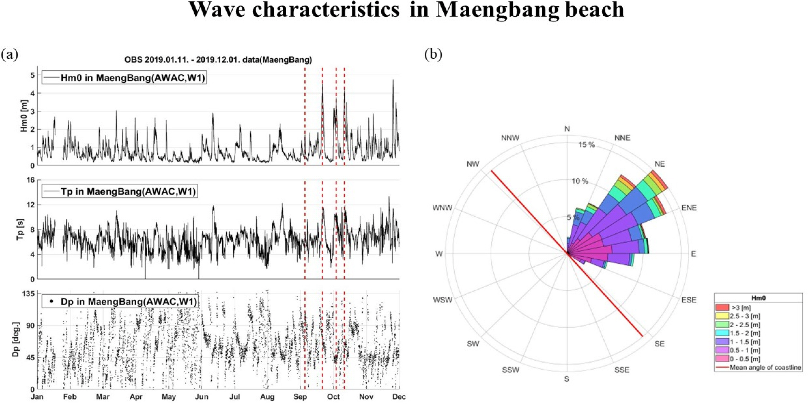
Wave characteristic in Maengbang beach: (a) Time-series of significant wave height (Hm0), peak period, and peak wave direction at W1 (red line: peak time of significant wave height for four typhoons that affected Maengbang beach); (b) Wave of significant wave height and mean wave direction rose in W1 with the mean angle of coastline.
Furthermore, the features of wave direction were distinctive according to the season. Therefore, overall, the average wave direction was 45°–90° in summer and 0°–45° in winter, which showed a fluctuation. High waves, the significant wave height of which was more than 3 m, were concentrated from September to December because of typhoons in summer and swell waves in winter.
Four typhoons (Lingling, Tapah, Mitag, and Hagibis), in particular, had direct or indirect impacts consecutively on the Korean Peninsula for around two months, through September 2019 and October 2019. Typhoon Lingling, the first typhoon in that period, affected the beach indirectly as it was going north to the West Sea; its significant wave height at the peak was only 1.7 m, the peak wave period was 10.2 s, and the peak wave direction was E, close to 90°. The most significant wave height during the four typhoons was 4.52 m at the time of Typhoon Tapah, the peak wave period was 10.2 s, and the peak wave direction was 69°. Typhoon Mitag was the only typhoon that passed directly through Maengbang beach. The significant wave height at the peak was 3.8 m, the peak wave period was 10.7 s, which was the highest value, and the peak wave direction was 42°, nearly perpendicular to the shoreline. The significant wave height during Typhoon Hagibis was 4.2 m, the second largest, the peak wave period was 10.5 s, and the peak wave direction was 53.4°. Table 1 summarizes the wave observation data at the time of the most significant wave height during the four typhoons. Fig. 3 shows the wave data schematized from August 29 to October 30 in 2019, the storm strike period, used as input data in XBeach in this study.
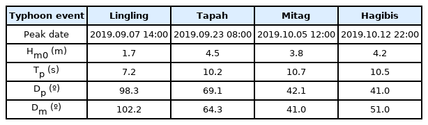
Summary of wave data during each typhoon from August 29 to October 30 in 2019
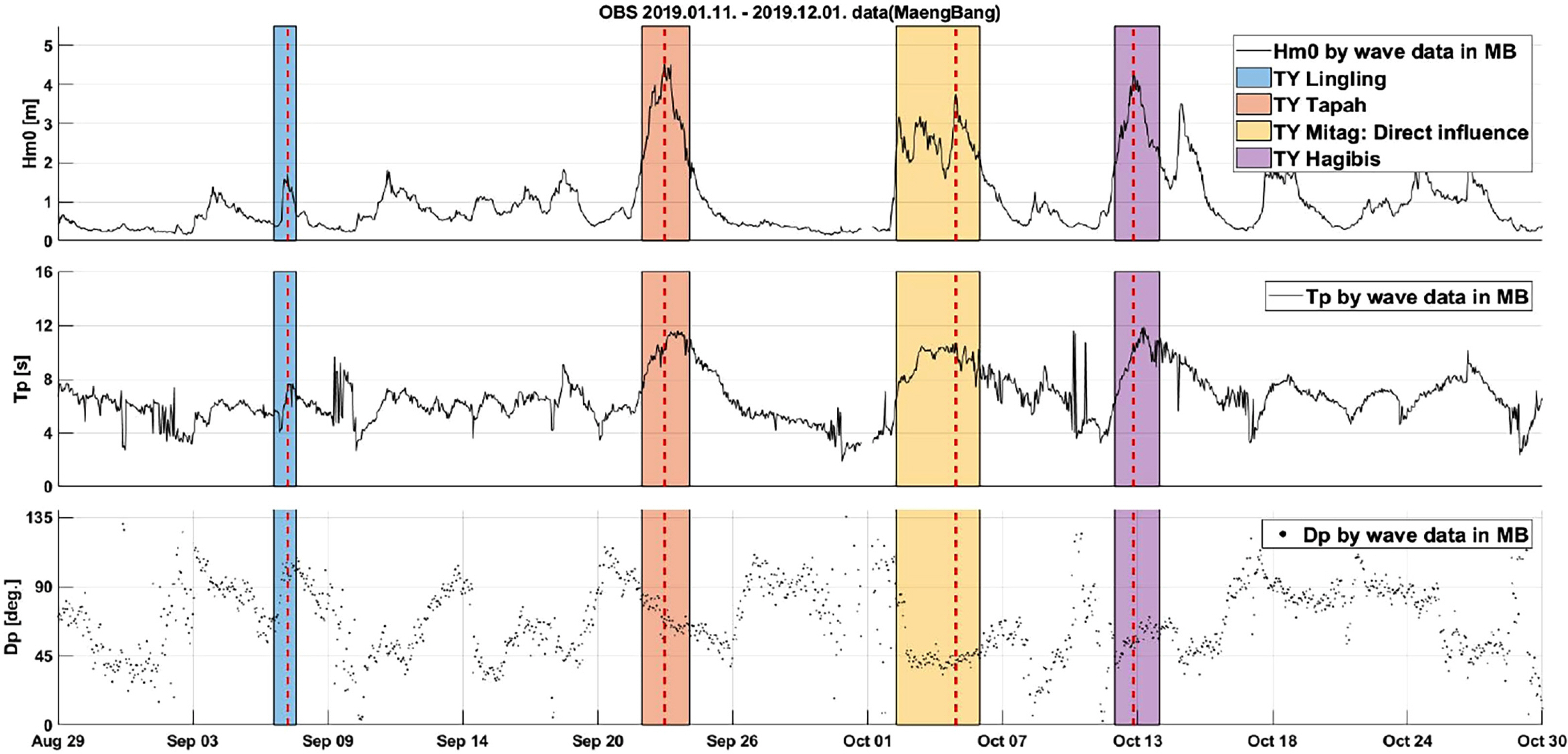
Observed wave data between August 29 and October 30 in 2019 (significant wave, peak period, peak direction) at AWAC (W1) (color boxes: each period affected by the typhoon).
2.4 Bed Elevation Data Before and After the Storms
The bed elevation was surveyed from Hanjaemit Beach to Deoksan Port at intervals of 50 m up to −25 m in the open sea, conducted eight times in 2019 to observe bed elevation and beach profile. The bed elevation was measured using an observation ship equipped with a global navigation satellite system (GNSS) and the AquaRuler 200 Series, a precision echo sounder. The beach profile survey was conducted up to the upper beach profile +6 m area using a real-time kinematic GNSS (RTK-GNSS), a virtual reference station method. The reliability of the observation data improved through comparison and calibration by overlapping some observation sections of the beach profile and bed elevation survey. Morphological changes were rarely observed outside the observed bed of −10 m. Thus, it was judged that the depth of closure of sand movement was in the vicinity. Although crescentic sandbars were repeatedly generated and removed within the littoral cell of Maengbang beach, the location of the sandbars was continuously maintained without significant change. However, as the sand in the surf zone moved in the open sea direction after the typhoon scenario that occurred in the summer of 2019, the curved shape of the crescentic sandbar changed into a longshore sandbar, stretched straight in parallel with the shoreline, and patterns of erosion and accretion appeared alternately in the shoreline. Figs. 4(a) and 4(b) show the bed elevation of Maengbang beach and formed crescentic and longshore sandbars on August 29 and October 30 in 2019, before and after the storm scenarios, respectively. Fig. 4(c) shows the closure depth of sediment transport and elevation difference before and after the storms. This study employed bed elevation data before and after the storms as input and calibration data to numerically model the erosion in the subaerial beach and the morphological changes in the dynamic surf zone due to the four continuous typhoons using XBeach.

(a) Bed elevation before the storms on August 29 in 2019 (white dash line: position of the crescentic bar), (b) bed elevation after the storms on October 30 in 2019 (white dash line: position of the longshore bar), and (c) The elevation difference between before and after the storms (red dash line: depth of closure with little sediment transport).
3. Configuration of the Numerical Model and Selection of Calibration Parameters
3.1 Numerical Simulation Grid Configuration and Introduction of Input Data
To consider all events directly or indirectly impacting a morphological change in Maengbang beach using the XBeach model, this study used the elevation on August 29, 2019, as the initial elevation, and the elevation on October 30, 2019, as the calibration data. The modeling period was somewhat as long as 63 days, which included all four typhoons. This long period may cause an exponential increase in numerical simulation time along with the long numerical simulation time of GLUE, which is a difficult problem to solve in GLUE due to the GLUE characteristics that numerically simulate many combinations of parameters. Thus, this study focused on reducing simulation time as much as possible when setting the model. The 2D Joint North Sea Wave Project (JONSWAP) spectrum was used on the basis of wave data provided by the AWAC mentioned in Section 2.3 to numerically simulate a wave-induced current as the offshore wave boundary condition, and only wave data with significant wave height greater than 2 m were used so as to reduce the simulation time. To consider the bed elevation caused by tide and storm surge, data from the Donghae Port Tide Station, the closest to the study area and provided by the Korea Hydrographic and Oceanographic Agency (KHOA), were used as the offshore water level boundary condition. The wave observation location (W1) in the AWAC was positioned around the edge of the open sea direction of the grid, as shown in Fig. 1(c), to avoid deforming the initial conditions of the waves within the model. The grid resolution was set to have a distance in the cross-shore direction narrowly in the concerned area (surf and swash zones), where morphological changes occurred relatively frequently, whereas the distance was made wider in the direction of the unconcerned area (open sea), where morphological changes rarely occurred, to reduce the simulation time. Curvilinear and non-equidistance grids (192 × 239 grids in cross-shore and alongshore directions) were created (Table 2). Additionally, a non-erodible layer option was applied to Deokbongsan or coastal roads, with the sediment thickness mentioned in a previous study that had a significant impact on simulation results (Do and Yoo, 2020).

Overview of XBeach grid
To simulate offshore fluid dynamic and morphodynamic processes during a storm, the currently widely used and proven surf-beat mode was used among many modes in XBeach that showed a difference in the hydraulic analysis of wave propagation. The surf-beat mode derives radiation stress after taking the offshore boundary conditions through the wave action balance equation from the perspective of group wave for short-period waves while using the nonlinear shallow water equation for long-period waves. Consequently, the surf-beat mode can simulate an infragravity wave motion, essential for water motion in the swash zone. The stationary mode, another option, can make calculations quicker as it interprets both short- and long-period components with the wave action balance equation. However, it has a limitation in accurately simulating sediment transport in the swash zone because it disregards the infragravity wave. On the other hand, the non-hydrostatic mode shows strength in simulation performance of sediment transport and morphological changes in all zones, including the swash zone, because it interprets both short- and long-period components using the nonlinear shallow water equation. However, it necessitates very long calculation times, thereby being unsuitable for field research. Finally, the message passing interface (MPI) was used in the calculation to obtain distributed and parallel processing with 36 nodes to reduce simulation time in the numerical simulation.
3.2 Selection of Wave Breaking and Sediment Transport Equations
XBeach contains various model equations usable to simulate morphological changes and sediment transport in the surf and swash zones. Thus, model users can select and apply equations on the basis of topographic characteristics or environment of the study area. Maengbang beach shows significant topographic variability in both cross-shore and alongshore directions because of the erosion and accretion patterns in the crescentic sandbar and shoreline, as aforementioned. Considering the characteristics of Maengbang beach, this study focused on a wave-breaking equation, which showed significant prediction performance sensitivity to nearshore elevation change, and the sediment transport equations, which exhibited excellent prediction performance by study area terrain and environment, among many types of equations. In the default setting of the latest XBeach version (XBeachX), Roelvink’s equation (Roelvink, 1993) is set for the wave-breaking equation, and the Van Thiel–Van Rijn equation (van Rijn, 2007a; van Rijn, 2007b) is set for the sediment transport equation. Roelvink’s equation experimentally and probabilistically estimates wave energy dissipation by wave breaking using Eqs. (1)–(3) (Roelvink, 1993). Here, the wave-breaking probability in Roelvink’s equation is an empirical formula type combined with the wave breaking coefficient (parameter gamma) and the ratio of wave height to water depth.
Here, D̄ω indicates the dissipation because of wave breaking, α indicates the wave dissipation coefficient, Qb indicates the wave-breaking probability, Eω indicates the wave energy, Trep indicates the represented wave period, Hrms indicates the RMS (Root-mean-square) wave height, Hmax indicates the peak wave height, and γ indicates the breaker index (gamma).
However, Daly et al. (2012) highlighted that Roelvink's equation underestimated the dissipation due to wave breaking in complex terrain with rapidly increasing water depth. To overcome this limitation, Daly's equation, the same as Roelvink's equation for others but determines whether wave breaking occurs by a binary value in the wave-breaking probability calculation, introduces an advective- deterministic approach whereby a wave-breaking characteristic advects into a wave speed, as presented in Eq. (4). Through this equation, wave breaking can be calculated in an on–off manner based on wave height even in a terrain where the water depth changes significantly.
Here, γ2 represents the threshold that determines whether wave breaking of irregular waves stops, which corresponds to parameter gamma2 in XBeach. Through various experimental data, Daly verified that Daly’s equation significantly improved wave-breaking prediction performance in a terrain where the water depth rapidly increased. On this basis, we determined that Daly’s equation was appropriate for Maengbang beach, regarded as complex water-depth terrain due to the continuous development of the crescentic sandbar. However, parameter gamma2 was also included in the wave-breaking equation, in contrast with Roelvink’s equation, taking more time in the calibration process.
Next, XBeach calculates sediment concentration using the water depth-averaged advection-diffusion equation (Eq. (5)) to simulate sediment transport (Galappatti and Vreugdenhil, 1985).
Here, C indicates the instantaneous concentration of the depth-averaged sediment, Dh indicates the diffusion of sediment, h indicates the water depth, uE and vE indicate the x and y components in the Euler flow velocity, Ceq indicates the equilibrium concentration of sediments, and Ts indicates the reaction time due to entrainment. The entrainment and sedimentation of sediments are determined on the basis of the difference between sediment instantaneous concentration (C) and sediment equilibrium concentration (Ceq), which becomes a source term of the sediment transport equation.
Here, Cmax represents the threshold of the maximum sediment concentration a user can set. The equilibrium concentration components of bed load and suspended load are needed to calculate the sediment equilibrium concentration (Eq. (6)). This equation can select the van Thiel–van Rijn equation, the default equation of the model, or the Soulsby equation (Soulsby, 1997; van Rijn, 2007c) according to the study sea. First, the van Thiel-van Rijn equation is as follows:
Here, Asb and Ass indicate the bed and suspended load coefficients, vmg indicates the Euler flow velocity, urms,2 indicates the empirical formula considering a turbulent flow due to orbital velocity and wave breaking, and Ucr indicates the threshold velocity of the sediment's initial movement, determined by the summation of weighted value after calculating the effects of sea current and waves separately. Additionally, the flow velocity of the sediment stirring in the sediment equilibrium concentration is a function of the infra-gravity wave, Euler's average flow velocity, and the wave's orbital velocity.
Next, the Soulsby equation considers the drag force coefficient by shear stress in the sediment stirring the velocity term, which is different from what the van Thiel-van Rijn equation says, to provide a relationship between the average flow velocity and bottom shear stress. It includes parameter z0, a length whereupon the bottom friction acts to represent the surface area whereupon the shear stress acts. Furthermore, sea current and wave are not separated when calculating Ucr, and the Soulsby equation is as follows:
Here, Cd represents the drag force coefficient and z0 represents the length whereupon the bottom friction acts, represented as the parameter z0 in XBeach. Furthermore, in the two sediment transport equations (Eqs. (9) and (10)) stated above, the entrainment and sedimentation of the sediments were represented from the perspective of the initial movement threshold of single particles. These two equations have been applied to seas and researched with many characteristics in previous studies. De Vet (2014) verified that the van Thiel–van Rijn equation showed better prediction performance of suspended load equilibrium concentration in a sea where overwash or breaching occurred than that which the Soulsby equation did. However, Orzech et al. (2011) revealed that a higher Brier skill score (BSS) was obtained when using the Soulsby equation of XBeach 2D modeling for beaches in Monterey Bay, USA, with rip channel and waveform shoreline (Megacusp) being features similar to those found on Maengbang beach. Pender and Karunarathna (2013) accurately reproduced the observation results through 1D modeling using the Soulsby equation during the storm at Narrabeen beach in Australia, a straight shore with a low tidal range environment, similar to the conditions prevalent on Maengbang beach. These previous studies implied that the sediment transport equation that showed the optimal performance differed depending on sea characteristics and environments. In our study, the Soulsby equation was selected as the sediment transport equation because it showed better prediction performance in conditions similar to those of Maengbang beach.
3.3 Selection and Rationale of the Calibration Parameters in the Numerical Model
In this study, resistance change according to changes in the dilatancy (pore volume) and bdslpeffdir (sediment transport direction adjustment) options were used out of the options in the experimental equation applied in De Vet (2014) to consider a process based on actual physical phenomena. Furthermore, dilatancy is known to improve model performance and mitigate excessive erosion in high flow velocity, considering the fluid pressure exerted on the inside of the sand because of changes in pore volume (De Vet, 2014; van Rhee, 2010). According to Talmon et al. (1995), bdslpeffdir applies a correlation in the sediment transport direction based on a bottom slope. Additionally, for the Chezy bottom friction coefficient, which improved the prediction performance of morphological change in the subaerial beach as it was known to reduce erosion when its value increased, this study used 40 m1/2/s, which showed a performance improvement when applied to Maengbang beach in a study by Jin et al. (2020), instead of using the model's default value (55 m1/2/s) (De Vet, 2014; Jin et al., 2020). Furthermore, for the median grain size (D50) in the XBeach model, assumed to be a single value in the model although a fine-grained distribution is found in the real, natural beach to the open sea, Jin et al. (2020) determined that the average value of the entire median grain size showed a better performance than the average value of the median grain size around the sea level in Maengbang beach did. Thus, the average median grain size of 0.4 mm of the entire water depth was used on the basis of analysis results of seabed conditions in Maengbang beach on August 29, 2019, where the initial water depth was observed before the storm strike. At the same time, although the morphological acceleration factor (morfac) showed an effect of highly reducing a simulation time in many studies on Xbeach for reducing simulation time, this study used morfac = 10, known to have low sensitivity to modeling results (Lindemer et al., 2010; Simmons et al., 2019; Vousdoukas et al., 2012).
Next, sensitivity and uncertainties were precisely analyzed through the systematic calibration of GLUE, and parameters that were expected to significantly improve in model performance were selected when choosing optimal parameters. As mentioned above, Maengbang beach is a region with significant alongshore variability in both the subaerial beach and underwater. The Daly equation, which improved the wave-breaking prediction in the sudden drop in water depth, is considered very important in improving prediction performance in nearshore modeling on the entire eastern coast of South Korea, including Maengbang beach, where the water depth rapidly changes due to the development of a crescentic sandbar. The parameter gamma is a threshold that determines when the breaking of irregular waves starts in the Daly equation. It is known that as the parameter value increases, dissipation due to wave breaking decreases. It has also been used frequently in several previous studies as a calibration parameter to improve morphological changes due to wave breaking (Daly et al., 2012; Harley et al., 2016; Jin et al., 2020; Kalligeris et al., 2020; Williams et al., 2012). Parameter gamma2 is also a threshold that determines when the breaking of irregular waves stops, thought to significantly contribute to the wave breaking prediction. However, few studies have been conducted on the sensitivity of model performance according to calibration when compared with gamma. Thus, we selected gamma2 along with gamma, which determines wave breaking, as calibration parameters. Moreover, the facua parameter exhibits the effect of sediment transport due to skewness and asymmetry of waves. Generally, the larger the value the more the sediment transport in the shoreline direction.
When calibrating Xbeach, facua requires a careful adjustment to improve prediction performance. And it is a parameter known to show the highest sensitivity, the reason why it has been mentioned as one of the main parameters in several previous studies (Bugajny et al., 2013; Cueto and Otero, 2020; Elsayed and Oumeraci, 2017; Harley et al., 2016; Kombiadou et al., 2021; Nederhoff et al., 2015; Orzech et al., 2011; Splinter and Palmsten, 2012; Vousdoukas et al., 2012). Furthermore, a previous study on the adoption of GLUE in the first numerical simulation results of XBeach also selected gamma and facua as calibration parameters to successfully improve performance. Thus, gamma, facua, and gamma2 were selected as the calibration parameters using GLUE. In this study, the initial parameter set of these three parameters was named the “INI set.” Table 3 summarizes the description of the used parameters and parameters to be calibrated through GLUE. Fig. 5 depicts the overall flow chart of GLUE. As shown in Fig. 5, the elements and ranges of parameters to be calibrated were first selected in the GLUE analysis, and then, parameter values were divided at regular intervals. Several parameter combinations made through this were numerically simulated, and based on the simulation results, a likelihood was calculated for each combination. Through this likelihood, sensitivity, likelihood probability density, and uncertainties were analyzed using the GLUE tool. In this study, two GLUE analyses were conducted; in the first sort phase, an entire range of parameters specified in the XBeach manual (Deltares, 2018) was considered toward selecting a precise range where prediction uncertainties were removed. In the subsequent precise phase, a range and a combination of optimal parameters that can maximize the numerical simulation performance were selected. More detailed descriptions and study results are sequentially described in Sections 4 and 5 (Fig. 5).
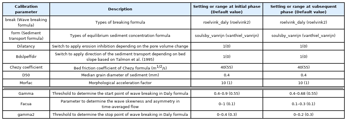
Description of the XBeach calibration parameter and setting/range of calibration at the initial and subsequent phase for GLUE
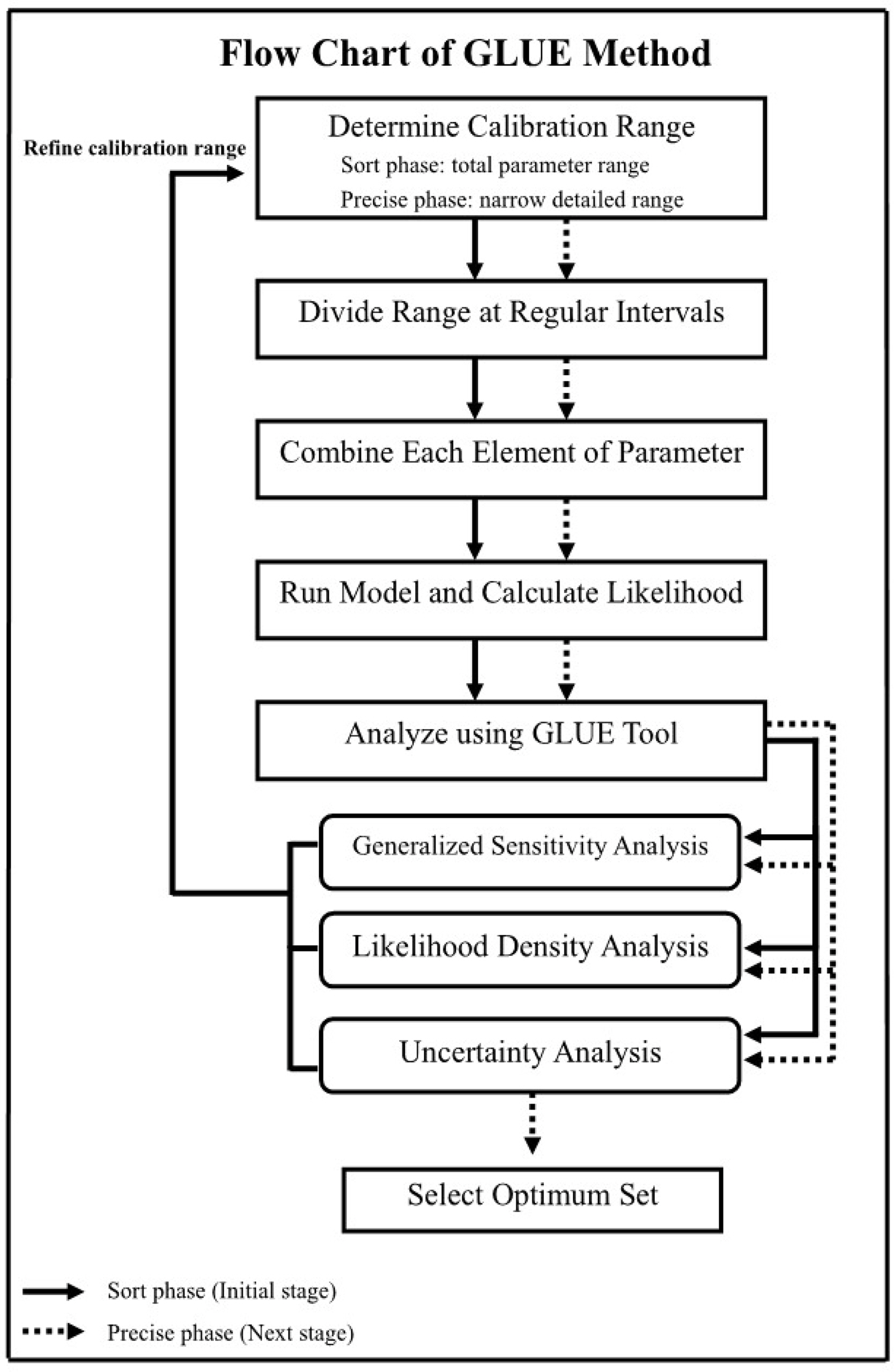
Flow chart of the GLUE process.
4. Selection of Initial Range of Parameters through GLUE
4.1 2D Calibration Method Assigned with Objectivity
The GLUE analysis overcomes the limitation of the existing trial-and-error method and assigns objectivity to calibration results. Thus, the entire range for each parameter was selected as the initial calibration area in the sort phase. Previous GLUE generated a random combination through Monte Carlo sampling when performing discretization of the set continuous range, but the current study generated a discrete combination at regular intervals to reduce the simulation time, which, otherwise, exponentially increased due to the combination of a long modeling period, 2D numerical simulation, and GLUE use. Thus, gamma was divided into six (0.4–0.9) at an interval of 0.1, facua was divided into 21 (0–1) at an interval of 0.05, and gamma2 was divided into five (0–0.4) at an interval of 0.1, thereby generating 609 INI sets to perform numerical simulation 609 times. The interval of facua was more finely divided as it affected sediment transport, and its importance during modeling was emphasized in a previous study. Because of the characteristic of the thresholds that started and stopped wave breaking, gamma, and gamma2 could not have the same parameter value. Therefore, 21 combinations with the same value were excluded from the initial 630 combinations.
In contrast with the previous studies on GLUE that were numerically simulated with 1D, a new 2D evaluation standard is required to consider the prediction performance of 2D simulation results. However, although much advancement in the improvement of erosion prediction performance during storms through parameter calibration on XBeach has been achieved with numerical models that showed erosion-dominant features, improvements in beach recovery and sedimentation prediction are yet to be achieved (Daly, 2017; Kombiadou et al., 2021). Thus, when conducting a 2D performance evaluation, if a dominant deposition profile is included, the evaluation index value is standardized downward, resulting in difficulties in quantitative evaluation. Considering this fact, this study selected a profile where beach regression or volume erosion was dominant as the baseline beach profile (hereafter referred to as the “baseline profile”) to be used as the evaluation standard. To comprehensively consider as many erosion profiles of many areas as possible, the baseline profile was selected so as not to let erosion profiles be adjacent to each other. Additionally, the profile erosion near No. 207 was attributed to the effect of Maeupcheon being located on the right-hand side, which was considered in that study. Thus, the profile was excluded in the selection of baseline profile. Fig. 6 shows the shoreline and volume changes that occurred on Maengbang beach before and after the typhoon scenarios. The four baseline profiles in the yellow lines were used in the first GLUE analysis. Subsequently, the three profiles in purple lines were added in the second GLUE analysis. Thus, seven baseline profiles were used as explained in Section 5. Furthermore, to consider the erosion in the subaerial beach, the importance of which has been stressed from the perspective of coastal disaster prevention, the swash zone (water depth of 0–4 m) was selected as the water depth at which to conduct performance evaluation.
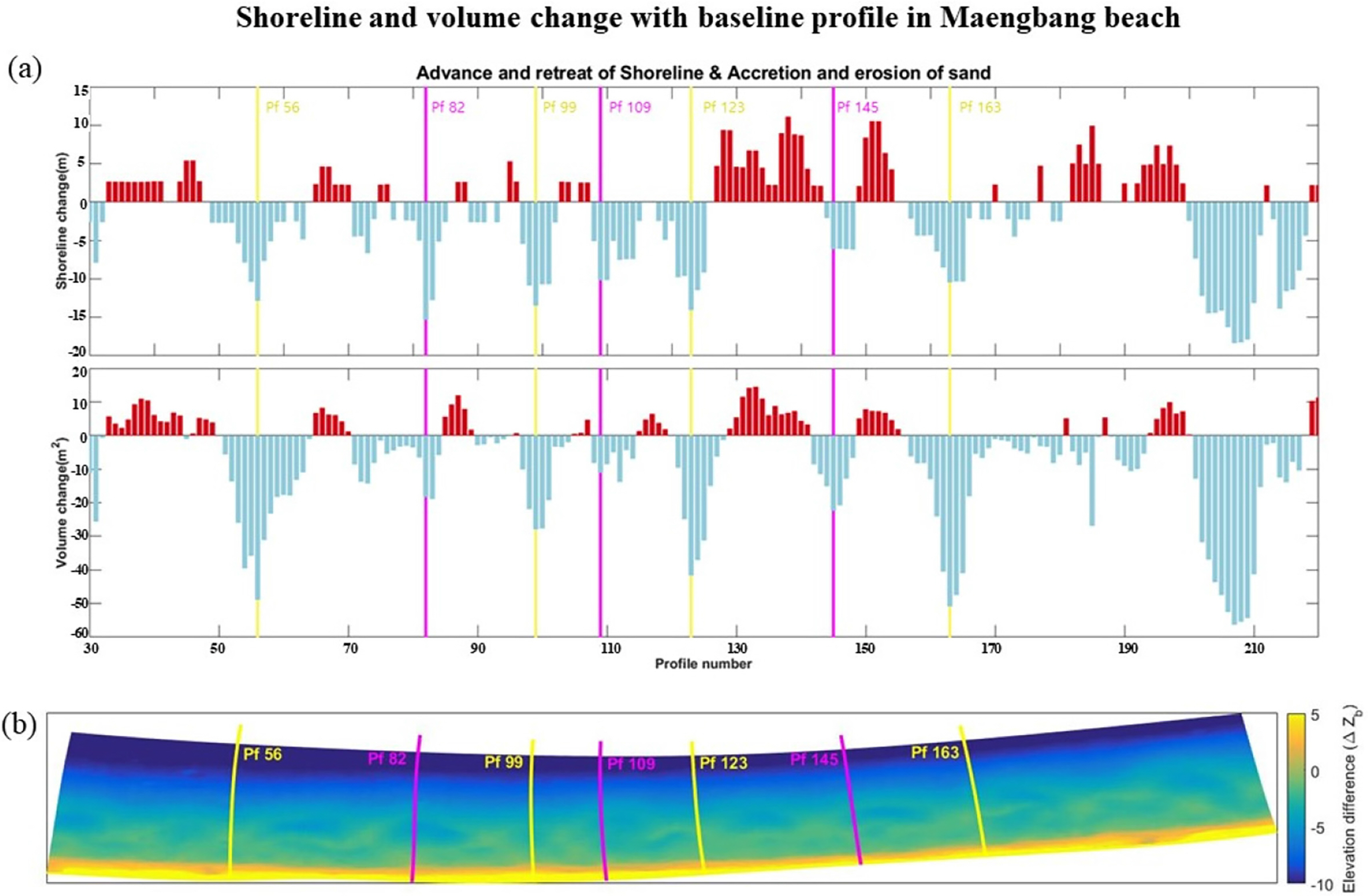
(a) Shoreline (up panel) and volume change (down panel) of each profile between before and after the storm in Maengbang beach, which represent progress/accretion (red bars), regress/erosion (blue bars), and baseline profile of GLUE [yellow lines: baseline profiles at sort phase (or initial phase: profile 56, 99, 123, 163), purple lines: additional baseline profiles at precise phase (or subsequent phase: additional profile 82, 109, 145)]; (b) Bed elevation before the storms with baseline profile in Maengbang beach.
BSS is an evaluation index used to closely review and evaluate a cross-sectional change in the prediction model proposed by van Rijn et al. (2003). It has been widely used as a significant quantitative standard for the prediction performance of numerical models in the field of coastal engineering. It is calculated by Eq. (12). In this study, the BSS shows how good the prediction performance of water depth after the storm is in comparison with the observed water depth after the storm based on the observed initial water depth as the evaluation standard.
Here, zm indicates the observed water depth after the storm, zp indicates the water depth result after the numerically simulated storm, zr indicates the water depth observed before the storm, which becomes the baseline water depth, t indicates the number of numerical simulations, and n (or N ) indicates the number of baseline profiles. BSS has a value between 0 and 1. The closer the value to 1 the better the prediction performance. And the closer the value to 0 the worse the performance. Table 4 presents the model performance according to the BSS values proposed in van Rijn et al. (2003).
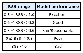
Qualification of model performance
As many simulation results must be processed due to the GLUE’s characteristics, it is necessary to have a certain quantitative standard to determine significant simulation results. Thus, a BSS threshold can be set based on the modeling objective and the model performance as measured by a BSS value. Based on this threshold, behavior and non-behavior were defined toward determining whether the simulation result of the combination showed a significant prediction. In this study, the behavior was defined as a combination, the average BSS value of which was derived by averaging BSSs in the baseline profiles for each parameter combination, was more than 0.3 (Eq. (13)).
Fig. 7 shows the average BSS values of the baseline profiles for each combination derived through the aforementioned process in the sort phase of GLUE. In this figure, combinations showing behavior were indicated in blue, combinations showing non-behavior in yellow, and combinations showing the maximum value in red. As shown in Fig. 7, unreasonable and low performances were mostly shown in the entire range of the parameters. Only some of the combinations showed a significant result, a behavior rate of approximately 10.18% (62 out of 609 profiles) because of the high sensitivity of model performance of facua in a certain limited range. The combination showing the maximum mean BSS was gamma = 0.9, facua = 0.1, and gamma2 = 0.1, which was 0.8429 of mean BSS. Other various combinations were also close to 0.84 of mean BSS. This implies that the equifinality displayed in a complex XBeach model was well identified through GLUE.
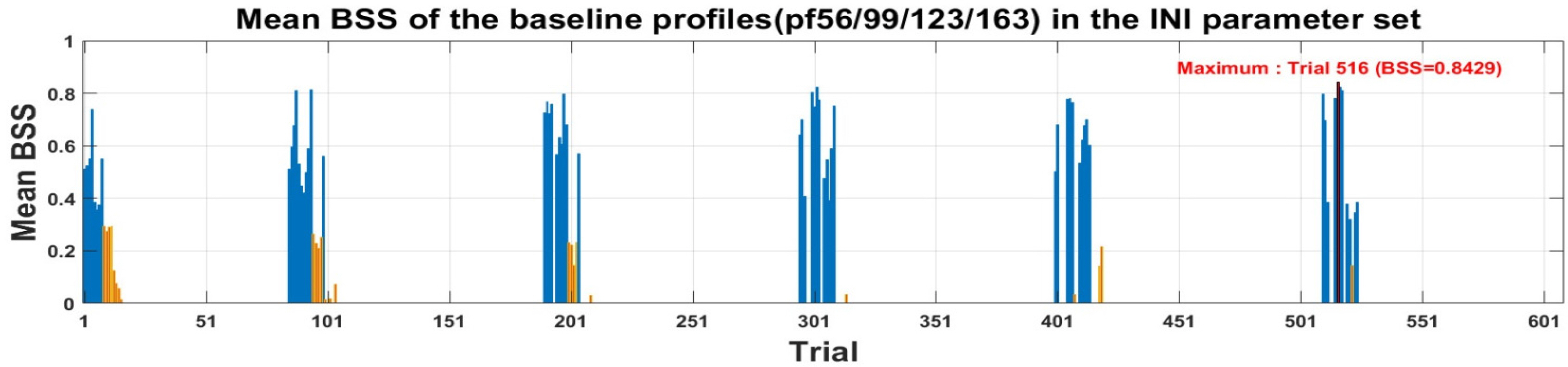
Mean BSS value of the erosion-dominated baseline profiles (profile: 56, 99, 123, 163) in INI set [red bar: trial number assigning maximum mean BSS value among all trials, blue bar: trial numbers of the behavioral run (BSS > 0.3), yellow bar: trial number of the non-behavioral run (BSS < 0.3)].
Afterward, to exclude the identified equifinality, a weighted likelihood calculated on the basis of BSS value was assigned to each combination and used as the standard of quantitative evaluation. A likelihood refers to the possibility that the used combination of parameters produces the optimal result when numerically simulating an observed event. Here, the likelihoods of all combinations of non-behavior defined above were set to 0, and the likelihoods of only the combinations of behavior were calculated using Eq. (14).
Here, n indicates the number of parameter combinations showing behavior, and BSSi indicates each BSS value of the combination showing behavior out of all parameter combinations. Based on this equation, likelihood indicates a proportion of one BSS value out of all BSS values. Thus, the likelihood of the combination will be small if the sum of BSS values derived in all combinations is large, even if the BSS value is derived high from a specific parameter combination, and the likelihood will be large if the sum of the derived BSS values is small. As such, if a likelihood is utilized, relative prediction performance can be considered to exclude equifinality. And it can be an evaluation index that can select a more significant combination out of all parameter combinations in a relative sense.
4.2 Selection of Likelihood-based Precision Range to Improve Prediction Reliability
Generalized sensitivity analysis (GSA), conducted through likelihoods assigned to the combinations of parameters, is a method for quantifying and evaluating the extent to which change in each parameter can partially affect the simulation result. In the GLUE, the GSA technique of Hornberger and Spear (1981) is extended to provide a ranking of sensitivity for each combination based on likelihood. This sensitivity analysis was performed using the difference between cumulative density function (CDF) and prior distribution function. Beven and Binley (1992) pointed out that setting a prior distribution, compared with CDF in the sensitivity analysis, with a wide range and uniform distribution function was suitable as the standard reference. Thus, this study assumed the prior distribution function with a continuous uniform distribution for all ranges of the parameters. Additionally, the Kolmogorov–Smirnov D statistic (K-SD) was used to quantify the difference between the CDF and continuous uniform distribution function (Thorndahl et al., 2008). K-SD shows the maximum value of the differences between the two functions. In the GSA, the closer the K-SD to 0 the smaller the sensitivity of the parameter to the simulation result, and the closer the K-SD to 1 the larger the sensitivity. The cumulative likelihood of each parameter value was diagrammed using a probability density function (PDF) to refine a range of parameters that showed significant performance in the study sea. The simulated result through the combination, including the parameter value, showed a more relatively significant prediction performance as the PDF value increased. Using this PDF and the relativity of likelihood, a range of parameters that can improve prediction performance and reduce uncertainties can be objectively selected.
Fig. 8 shows the diagrams of CDF and PDF of the INI set, analyzed through the above description. As shown in Fig. 8, in the GLUE sort phase, the highest sensitivity was shown as K-SD = 0.86254 when facua was 0.1, K-SD = 0.23176 when gamma2 was 0, and K-SD = 0.10468 when gamma was 0.4. Although the sensitivities of gamma and gamma2 tended to decrease as the parameter value increased, likelihoods showed relatively uniform accumulation. However, the sensitivity of facua rapidly increased in a low parameter value so that combinations using values greater than 0.15 showed non-behavior that did not show a significant prediction performance as their cumulative likelihood value was 0. Additionally, the maximum PDF value was shown when facua was 0.05 and the cumulative BSS value was 15.0567, showing a sole trend of PDF concentration in a limited range (0–0.15). The maximum PDF value was exhibited when gamma was 0.7, and the cumulative BSS value was 7.6553. The maximum PDF value was exhibited when gamma2 was 0.1, and the cumulative BSS value was 9.2277, showing a PDF shape distributed over all ranges. As the maximum PDF value was shown differently depending on the number of first discrete parameter values, direct comparison between gamma and gamma2 was limited (gamma: six discrete values, gamma2: five discrete values). However, the maximum PDF value of facua was higher even when the number of discrete numbers was approximately four times greater than that of the two parameters mentioned above (facua: 21 values). This implies that calibrating at fine intervals of facua is critical when modeling the region, and the excessive erosion of XBeach can be appropriately avoided by carefully adjusting the sediment transport direction via facua.

Schematized cumulative distribution function (upper panel) and likelihood probability distribution function (bottom panel) for INI set (upper panel: blue line – cumulative likelihood function of a behavioral run at INI set, red dash line – uniform prior distribution function at INI set; bottom panel: blue dash line – the parameter value showing the maximum BSS of the parameter range, red dash line – parameter default value of model).
Through the sort phase of the GLUE in the foregoing discussion, sensitivities of each parameter and a range that showed behavior can be identified, and a range of non-behavior, the prediction uncertainty of which was largely owing to a low likelihood, can be excluded. Through the later GLUE analysis in the precision phase, a precision range of parameters was refined to propose the optimal combination of parameters. The range of gamma was refined to 0.4–0.68 at 0.04 intervals as the parameter values, where the K-SD and maximum PDF values derived were 0.4 and 0.7, respectively, located relatively far from each other. As the values where K-SD and the maximum PDF value were derived in facua were relatively close, the precision range of facua was set to 0.05–0.3 at 0.025 intervals. For gamma2, the precision range was refined to 0–0.2 at 0.04 intervals. A total of 528 refined parameter sets were named “RE set” in this study, and numerical simulations were performed 528 times again.
5. Proposal of Optimal Range and Combination with the Precision Range through GLUE
5.1 Calculation of Optimal Range Based on Likelihood to Improve Prediction Performance
To identify the outline of the combination of significant performance and applicability of GLUE on 2D simulation results of Maengbang beach in the sort phase, four baseline profiles (Profile 56, 99, 123, and 163) were adopted as the evaluation standard for the erosion-dominant characteristics of the XBeach model. In the precision phase of GLUE, three profiles (Profile 82, 109, and 145) were added to the existing baseline profiles, as shown in Fig. 6, to improve the alongshore evaluation performance, and the swash zone (0–4 m of water depth) was maintained as the evaluation water depth. Thus, although non-behavior showed a higher appearance rate overall, 161 out of 528 parameter sets showed behavior (BSS ≥ 0.3), which showed approximately 30.49% of behavior rate. This was a significantly improved behavior rate when compared with approximately 10.18% in the sort phase, which suggests that the range of behavior sets can be refined through repetitive GLUE analysis. The maximum BSS value was exhibited out of all sets when gamma = 0.64, facua = 0.075, and gamma2 = 0.16, and its mean BSS = 0.6891. The somewhat lower BSS compared to that of the sort phase due to the effect of the added baseline profiles. Fig. 9 schematizes the CDF and PDF in the analyzed RE set. According to Fig. 9, when facua was 0.1, K-SD = 0.7231, which showed the maximum sensitivity, and when gamma2 was 0, K-SD = 0.17992, and when gamma was 0.4, K-SD = 0.10932. All three parameters derived the maximum sensitivity from the same parameter values, and the large and small relationships were also maintained, producing the largest sensitivity in facua, followed by gamma2 and gamma. The refined precision range resolved the trend of limiting the sensitivity of facua to a specific value only to some extent compared to that of the initial range. However, it still showed a trend of sensitivity concentrated on 0.1 or lower. Thus, careful adjustment of facua is still required during calibration.
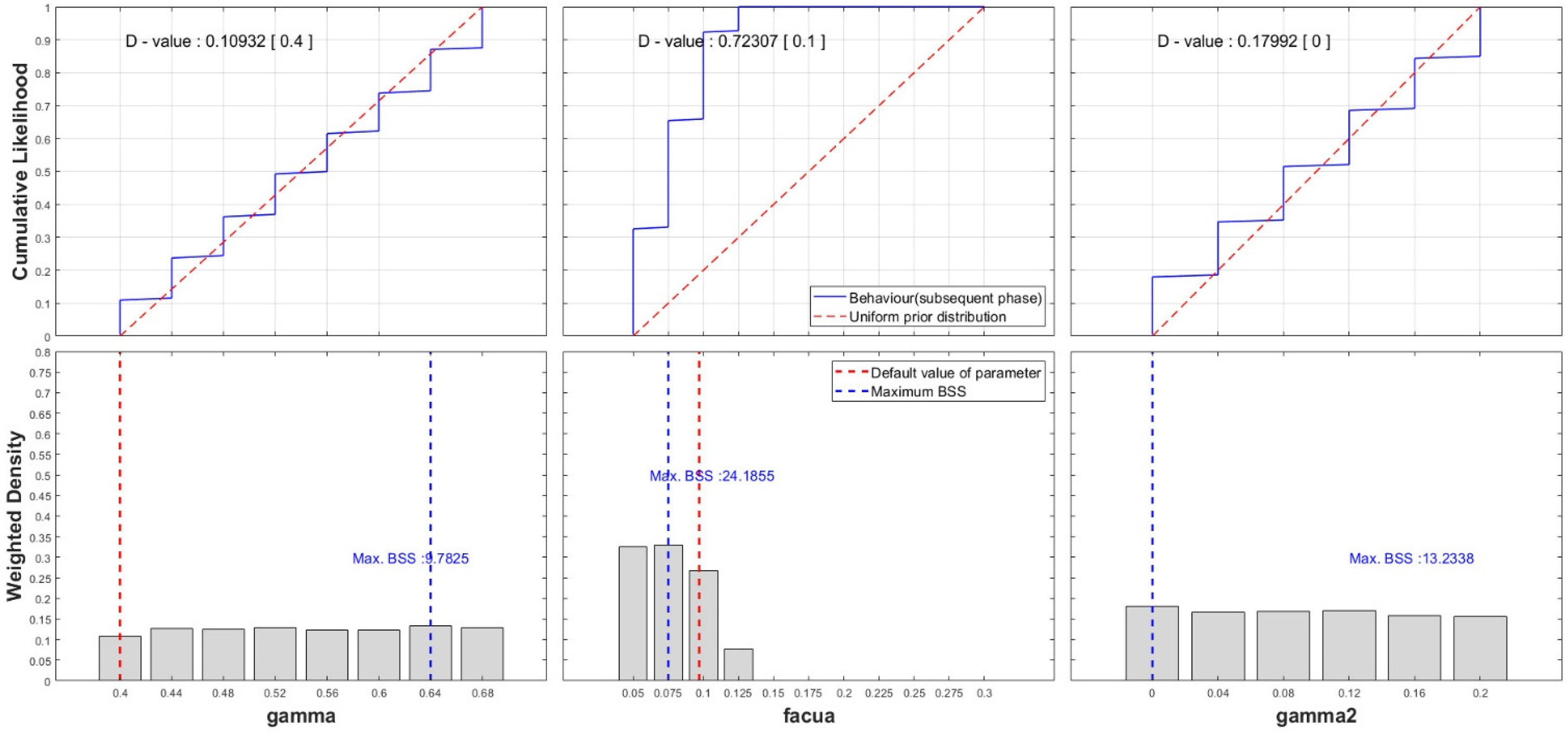
Schematized cumulative distribution function (upper panel) and likelihood probability distribution function (bottom panel) for RE set (upper panel: blue line – cumulative likelihood function of a behavioral run at RE set, red dash line – uniform prior distribution function at RE set; bottom panel: blue dash line – the parameter value showing the maximum BSS of the parameter range, red dash line – parameter default value of model).
When facua was 0.075, the PDF was 0.3288, significantly higher than the other two parameters. The maximum PDF value was calculated, which was higher than that of the sort phase. When gamma was 0.64 and gamma2 was 0, the maximum PDF value was revealed, indicating a tendency for a slightly lower maximum PDF value than that in the sort phase. PDF was more leveled through the repeated GLUE analysis than it was in the sort phase, but the derived maximum cumulative BSS value increased. This was due to the improved performance and reduced uncertainties by the refined prevision range in Maengbang beach. This implies that if GLUE calibration is continuously repeated, the optimized range that can be universally used while minimizing uncertainties can be derived.
Furthermore, the gamma and gamma2 parameters, which produced relatively leveled PDF, represented wave breaking and will show higher sensitivities due to alongshore variability, such as a water depth by beach profile, than that shown by facua, which reflected wave asymmetry. Thus, the leveled PDF was revealed because of the larger effect of the evaluation method that averaged BSSs of all baseline profiles adopted in this study. To overcome this issue, a measure of a solution is required, in which the profile-specific calibration mentioned in Simmons et al. (2019) can also be applied to the 2D simulation results. Note that the parameters used to derive the maximum K-SD and maximum PDF values did not necessarily match, indicating that high sensitivity did not directly correlate with the performance of simulation results. After completing the calibration, optimal performances were shown when facua was lower and gamma was higher than the default value in the model (Fig. 9). This was due to the physical characteristics included in the parameters. For example, when gamma increased, wave breaking increased, and wave energy dissipation decreased due to the increase in the threshold of wave-breaking generation. Therefore, wave energy reaching the shoreline increased, which increased erosion near the shoreline. However, when facua decreased, sediment transport decreased in the shoreline direction, increasing erosion near the shoreline. In this regard, gamma and facua were calibrated in the direction that can improve the excessive erosion in XBeach, which is consistent with the findings of previous studies (Elsayed and Oumeraci, 2017; Simmons et al., 2019). Table 5 summarizes the quantitative evaluation results of sensitivities and likelihood probability analysis in the sort and precision phases of GLUE performed in Sections 4 and 5.
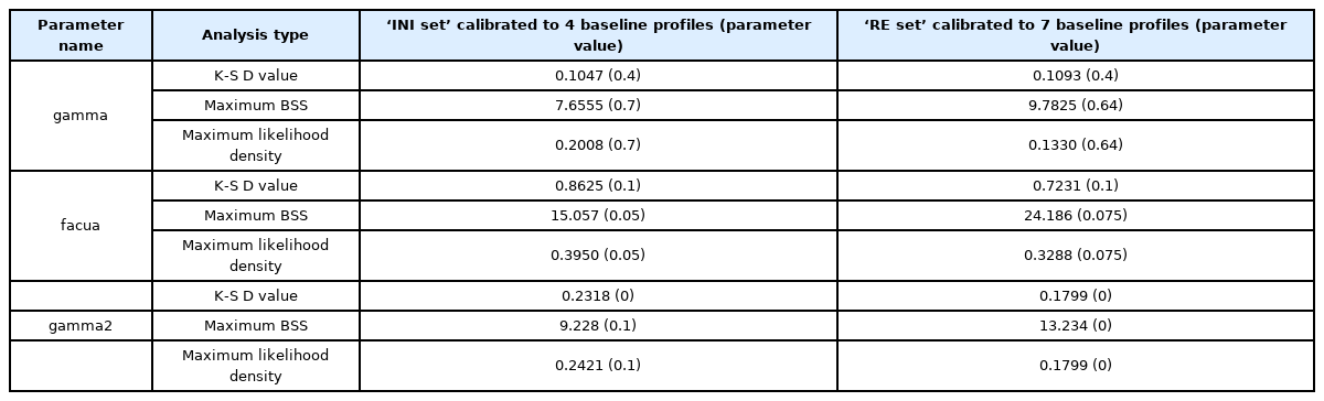
Calculated quantitative analysis values (K-S D value, Maximum BSS, Maximum likelihood probability density value) of simulated result in sort and precise phase. A value in the bracket is the parameter value from which the analysis value is derived.
5.2 Limitation of baseline profiles and performance evaluation to select optimal combinations
The parameters can be quantitatively analyzed, and the optimal ranges of parameters that reduce uncertainties can be selected through a sequentially conducted GLUE analysis. However, this process was an evaluation method considering only some erosion-dominant profiles out of all profiles to suppress the downward leveling of quantitative evaluation results owing to the characteristics of XBeach during GLUE analysis. Hence, we are skeptical about the calibration result from the swash zone (water depth 0–4 m) of seven baseline profiles and whether it can represent the entire study sea. Thus, we conducted GLUE calibration in the precision phase one more time with the evaluation standards, considering most profiles and water depths in Maengbang beach and the baseline profiles. As a result, only one out of 528 combinations showed behavior, which was gamma = 0.68, facua = 0.1, and gamma2 = 0.04. Its average BSS value was 0.321; this combination was named “COMB3.” Furthermore, the optimal combination selected through seven baseline profiles in Section 5.1 was gamma = 0.64, facua = 0.075, and gamma2 = 0.16. Its average BSS was 0.6891 and was named “COMB1” in this study. Next, the result that combined parameter values and that showed that the cumulative likelihood values were the highest for each parameter among the analysis results obtained in Section 5.1 was gamma = 0.64, facua = 0.075, and gamma2 = 0. Its average BSS value was 0.5826 and was named “COMB2.” Finally, to examine the entire region of Maengbang beach without using the baseline profiles, calibration evaluation standards were set to the beach profiles (Profiles 30–200) in the center of the beach and the surf and swash zones (water depth −8–4 m) to average BSS values derived in their profiles. Table 6 summarizes the calibrated parameter combinations and performance evaluation results using GLUE.
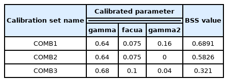
Calibrated parameter and calculated maximum BSS value for optimum 2D numerical modeling result at Maengbang beach
Fig. 10 schematizes the measured morphological change before and after a series of storms on Maengbang beach and 2D numerical modeling results of three calibrated combinations, in which the solid red line indicates the baseline profile. As shown in Fig. 10, both COMB1 and COMB2 simulated the erosion at a water depth of −5–−2 m in the surf zone and accretion at a water depth of −8–−5 m relatively well and successfully simulated the longshore sandbar, parallel to the shoreline formed after the storm strike. However, COMB1 showed a trend of relatively overestimated erosion and accretion in the surf zone compared to the observed values, whereas the accretion at a water depth of −2–0 m was underestimated. As a result, the error of erosion and accretion in COMB2 was relatively alleviated compared to that of COMB1. However, it also revealed a limitation in accurately predicting locations of erosion and accretion compared to the observed values. The alleviation of erosion and accretion error in COMB2 compared to COMB1 was because of gamma2, which indicated a correlation between gamma2 value and erosion and accretion at the surf zone. When gamma2 increased, it generated a wave-breaking stop more quickly as the breaking wave entered from the sandbar crest into the sandbar trough, which reduced the sediment transport and erosion caused by the breaking wave at a water depth of −5–−2 m. Additionally, COMB1 and COMB2 did not simulate the erosion and accretion patterns in the shoreline due to the overestimation of erosion near the shoreline as the location of the longshore sandbar formed at a water depth of −8–−5 m was produced in the open sea direction, farther than the observed value. This was because erosion-dominant baseline profiles were considered the evaluation standard.
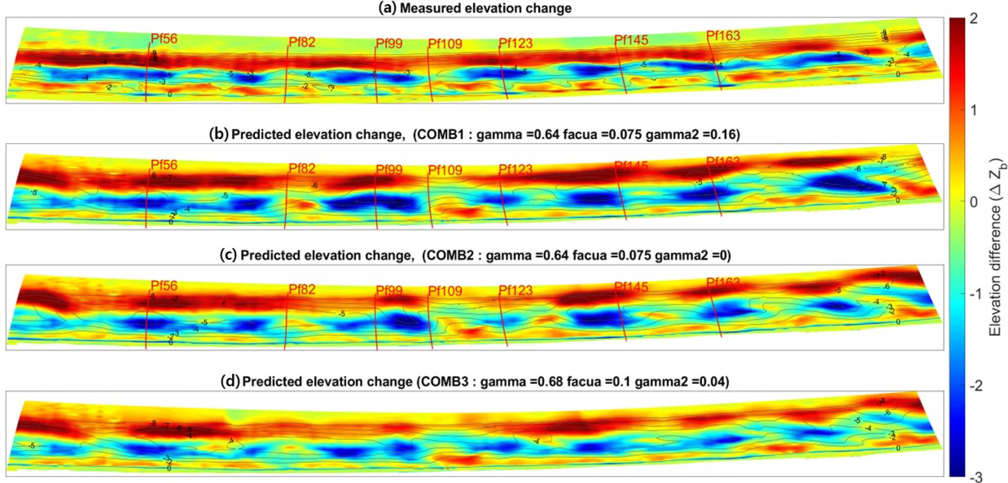
(a) Measured morphologic change between before and after a series of storms. (b) Predicted morphologic change using COMB1 in XBeach. (c) Predicted morphologic change using COMB2 in XBeach. (d) Predicted morphologic change using COMB3 in XBeach.
COMB3 exhibited a reduced erosion pattern near the left-hand side and central shoreline of Maengbang beach compared with COMB1 and COMB2, and the excessive erosion at a surf zone of −5–−2 m, as shown in Figs. 10(b) and 10(c), was considerably alleviated. This implies that the performance evaluation using erosion-dominant baseline profiles can induce excessive erosion. Moreover, COMB2 accurately simulated the accretion in the longshore sandbar formed at a water depth of −8–−5 m. Thus, the overestimated accretion at a water depth of −2–−0 m, which was revealed in COMB1 and COMB2, was considerably alleviated. However, the location of the longshore sandbar at a water depth of −8–−5 m was still somewhat deviated from the open sea, and the repeated erosion and accretion pattern was not simulated well although the erosion near the shoreline was alleviated. Furthermore, a considerable error was produced on the right-hand side in the simulation results of Maengbang beach because the effect of Maeupcheon and sediment transport was not considered in the modeling.
In summary of the above results, when calibrating the 2D numerical modeling, the combinations of the parameters derived from the erosion-dominant baseline profiles induced excessive erosion and accretion in the surf zone and excessive erosion near the shoreline. These limitations were significantly alleviated through calibration that considered many profiles and water depths, but selecting many profiles and water depths as the evaluation standard from the start of GLUE still exposed limitations due to the downward leveling of the evaluation results caused by the characteristics of the XBeach model. Thus, the optimal range that excludes uncertainties using two GLUE analyses is first calculated through erosion-dominant baseline profiles, and then, applying many profiles and water depths when selecting the final optimal combinations will significantly improve the calibration performance of the 2D simulation results.
6. Conclusions
We improved the unsystematic and passive drawbacks of the trial-and-error method, generally used for parameter calibration to improve the performance of XBeach, a nearshore morphological change model. We also simulated nearshore morphological changes on the eastern coast of South Korea using GLUE, a systematic calibration technique that can exclude uncertainties inherent in nearshore models. The study area was Meangbang beach, which showed typical characteristics of the eastern coast of South Korea, and four consecutive typhoons struck in 2019. Maengbang beach experienced considerable beach erosion and morphological changes in the surf zone during the storms. Additionally, the crescentic sandbar and arc-shaped beach, which are morphological features of the eastern coast of South Korea, are well developed. Thus, it is a place where a considerably complex nearshore process occurs due to the large alongshore variability and water-depth changes. This study employed a 2D JONSWAP spectrum of wave data that satisfied 2 m or higher significant wave height condition as the offshore wave boundary condition. For the offshore water level boundary condition, data from the Donghae Port Tide Station were used to numerically simulate the study area while reducing the long simulation time of GLUE. Curvilinear and non-equidistance grids (192 × 239 grids in the cross-shore and alongshore directions), whose resolution was higher in the longshore direction. The Daly equation, which improved the wave-breaking prediction performance in regions where the water depth rapidly dropped, and the Soulsby equation, which showed a good prediction performance of sediment concentration in beaches that were like Maengbang beach, were set as wave-breaking and sediment transport equations. For the parameters, dilatancy and bdslpeffdir were applied, which are options in the experimental equation based on physical phenomena that alleviate the erosion. Furthermore, Chezy = 40 m1/2/s and D50 = 0.4 mm were used, which showed a good performance of numerical simulation of Maengbang beach in a previous study (De Vet, 2014; Jin et al., 2020). Furthermore, the morphological change acceleration factor was set as 10 to shorten the simulation time. For the systematic calibration parameters used to analyze uncertainties through GLUE, parameters gamma and gamma2, which were included in the Daly equation that considerably improved a wave-breaking prediction based on a rapid change in water depth, as shown in Maengbang beach, and parameter facua, which was widely known as the importance of sediment transport prediction in a previous study, were selected. The 609 initial combinations (INI set) of the parameters were generated in the sort phase by combining discrete parameters at regular intervals when applying GLUE, and 528 combinations of the parameters (RE set) were generated in the precision phase to conduct sensitivity and likelihood probability density analysis. We also conducted 2D numerical simulations, which were in contrast with previous GLUE studies. Thus, we needed a standard to comprehensively evaluate many profiles. Four profiles whose erosion was the most dominant were nominated as the baseline profiles and used as the evaluation standard, considering the erosion-dominant characteristics of XBeach. Four BSS values of water depth 0–4 m in the profiles were calculated and averaged. The CDF and PDF were evaluated through the likelihood calculated in the behavior whose average BSS value was 0.3 or higher, and the result in the sort phase of GLUE (the first analysis) indicated that when facua was 0.1, K-SD = 0.86254, when gamma2 was 0, K-SD = 0.23176, and when gamma was 0.4, K-SD = 0.10468 in Maengbang beach. Furthermore, facua exhibited the highest sensitivity. In contrast, gamma and gamma2 showed relatively even behavior in all ranges in terms of PDF, while facua was concentrated on 0–0.1, showing non-behavior if it exceeded 0.15. Thus, it is essential to finely adjust facua when modeling Maengbang beach, through which excessive erosion of XBeach can be alleviated. The precision range of the parameters was refined based on the CDF and PDF in the sort phase as follows: gamma was 0.4–0.68 at 0.04 intervals, facua was 0.05–0.3 at 0.025 intervals, and gamma2 was 0–0.2 at 0.04 intervals. The GLUE analysis was conducted by generating 528 combinations and numerically simulating them. Here, four baseline profiles in the sort phase were expanded to seven in the precision phase (the second analysis) to create a more valid model performance evaluation standard. As a result, in the precision phase, Maengbang beach produced K-SD = 0.7231 when facua was 0.1, K-SD = 0.17992 when gamma2 was 0, and K-SD = 0.10932 when gamma was 0.4, demonstrating that facua revealed much higher sensitivities as shown in the sort phase. PDF was relatively leveled compared to that of the sort phase, but the cumulative BSS value in the parameter value increased, implying that a range that was improved further and reduced uncertainties in Maengbang beach would be suggested through the GLUE analysis. Thus, by repeating the GLUE calibration, a range that can be universally applied to the study sea can be selected. Furthermore, gamma and gamma2 showed a more even likelihood distribution than facua. This was because gamma and gamma2 were more affected by the alongshore direction variability in Maengbang beach than facua. Therefore, when proposing universal parameters in the study sea through GLUE, the selection of gamma and gamma2 is limited, and if facua is selected in the range of 0.05–0.1, it will produce a good prediction performance in Maengbang beach. Furthermore, GLUE calibration was conducted to alleviate the excessive erosion in XBeach, yielding the maximum cumulative likelihood when facua was 0.75 and gamma was 0.64. Through these quantitative evaluations, COMB1: gamma = 0.64, facua = 0.075, and gamma2 = 0.16 (BSS = 0.6891), which finally showed the highest average BSS value, and COMB2: gamma = 0.64, facua = 0.075, and gamma2 = 0 (BSS = 5826), which combined parameter values showing the maximum cumulative likelihood in each parameter, were selected as candidates of optimal parameter combinations in Maengbang beach, thereby comparing the 2D simulation results. Furthermore, the difference in calibration performance between using partial baseline profiles of Maengbang beach and using many continuous profiles as the evaluation standard was compared. To achieve this, the surf and swash zones (water depth of −8–4 m) in the center of the beach (profiles 30–200) were set as the evaluation standard of calibration, and COMB3: gamma = 0.68, facua = 0.1, and gamma2 = 0.04 (BSS = 0.321), which solely showed behavior, were also compared. Therefore, COMB1 and COMB2 successfully formed the erosion and accretion pattern in the surf zone of Maengbang beach and the longshore sandbar after the storm. However, the erosion and accretion at a water depth of −8–−2 m were relatively overestimated compared to the observed value, and the erosion at a water depth of −2–0 m was underestimated. COMB2 exhibited an alleviated error with the observed value compared to that of COMB1, which was due to the quicker wave breaking when breaking waves progressed from the sandbar crest to the trough as gamma2 increased, thereby reducing the sediment transport and the erosion in the surf zone caused by the breaking waves. COMB3 also accurately simulated the pattern of erosion and accretion, as well as the formation of the longshore sandbar on Maengbang beach. The error with the observed result, in particular, was more alleviated than that of COMB1 and COMB2. However, it still showed a limitation in producing an accurate location of the longshore sandbar and simulating an erosion and accretion pattern in the shoreline. Because using only erosion-dominant baseline profiles as the evaluation standard caused the increase in erosion in the overall simulation results, two GLUE analyses were conducted to calculate the optimal range, and finally, the optimal combination was selected. At this time, it would be more suitable to apply evaluation standards that can consider most of the profiles. This study required a considerable numerical simulation time because of the relatively long modeling period of 63 days and the use of 2D numerical simulations. Accordingly, many conditions were included to reduce simulation time, and the number of numerical simulations was smaller than that of the 1D GLUE study. Nonetheless, our study contributed to the applicability of 2D modeling using GLUE, quantitative performance evaluation of nearshore modeling on the eastern coast of South Korea, and analysis of uncertainties. If future studies apply various parameters and eastern coasts, it is considered that it can improve the reliability of nearshore modeling on the eastern coasts of South Korea through GLUE.
Notes
No potential conflict of interest relevant to this article was reported.
This study was supported by a This study was supported by the National Research Foundation of Korea grant funded by the Korea government (NRF-2022R1I1A3065599), and by the project titled “Establishment of the Ocean Research Station in the Jurisdiction Zone and Convergence Research” funded by the Ministry of Oceans and Fisheries in Korea.