Analysis of Steady Vortex Rings Using Contour Dynamics Method for Fluid Velocity
Article information

Abstract
Most studies on the shape of the steady vortex ring have been based on the Stokes stream function approach. In this study, the velocity approach is introduced as a trial approach. A contour dynamics method for fluid velocity is used to analyze the Norbury–Fraenkel family of vortex rings. Analytic integration is performed over the logarithmic-singular segment. A system of nonlinear equations for the discretized shape of the vortex core is formulated using the material boundary condition of the core. An additional condition for the velocities of the vortical and impulse centers is introduced to complete the system of equations. Numerical solutions are successfully obtained for the system of nonlinear equations using the iterative scheme. Specifically, the evaluation of the kinetic energy in terms of line integrals is examined closely. The results of the proposed method are compared with those of the stream function approaches. The results show good agreement, and thereby, confirm the validity of the proposed method.
1. Introduction
A water-jet can be used as one of the propulsion systems for ships and marine life. When a jet is injected to obtain thrust, a vortex ring is formed at a nozzle and then propagated downstream (Krueger et al., 2008). Furthermore, a vortex ring is generated due to volcanic eruption or nuclear explosion (Akhmetov, 2009).
The flow of a vortex ring is formulated with the Helmholtz vorticity equation in inviscid and incompressible fluids (Batchelor, 1967). A steady vortex ring was first reported by Helmholtz (1867) who examined a vortex ring of an small circular cross section, while a spherical vortex was first analyzed by Hill (1894). Norbury (1973) analyzed a vortex ring in a steady state for general circumstances, which is referred to as the Norbury–Fraenkel family (N-F family) of vortex rings.
A dynamic analysis is required for analyzing the instability due to the disturbance or interaction between vortex rings. A contour dynamics (CD) method for fluid velocity is used for analyzing the complex evolution of the contour of a vortex core. The CD method is a two-dimensional or axisymmetric flow analysis method due to the isolated vorticity in an inviscid, incompressible, and irrotational flow field (Pullin, 1992; Smith et al., 2018). The CD method can drastically reduce the burden of computations because the computation is performed in the form of line integrals on the boundary contour of the vorticity region. The fluid velocity on the contour is calculated using the CD method and then applied with time integrals to estimate the dynamic changes in the shape of the vortex core. Zabusky et al. (1979) introduced the CD method in dynamic analysis of two-dimensional vortex patches. Various examples of dynamic analysis for three- dimensional axisymmetric vortex rings are provided in the study by Shariff et al. (1989).
In this study, the CD method was applied to the analysis of the N-F family of vortex rings which are flows in steady state. Choi (2020) combined the CD method for a stream function (Shariff et al., 1989) and the direct shape-calculation method, and thus obtained results that were superior that those reported by Norbury (1973) wherein surface integrals and Fourier analysis were used. As a follow-up study to Choi (2020), in this study, we analyzed the N-F family of vortex rings using the CD method for fluid velocity examined in studies by Shariff et al. (1989) and Shariff et al. (2008). A stream function has been mostly used for analyzing a vortex ring in a steady state (Batchelor, 1967; Fraenkel, 1970; Fraenkel, 1972; Norbury 1973). In this study, we examined whether the CD method for fluid velocity, which is used in dynamic analysis, can also be applied to the analysis of a vortex ring in a steady state.
By applying the boundary conditions of a vortex core to the fluid velocity determined via contour integral, we proposed nonlinear simultaneous equations for the forward speed of a vortex ring and core shape nodal points. The shape nodal points and forward speed were determined via iterative calculations by applying an additional conditional equation, which specified that the speed of vortex center and impulse center were the same. The characteristics of core shapes and vortex rings proved that the analytical method used in this study is valid based on the comparison with previous results.
2. Problem Formulation
The fluid is assumed as inviscid and incompressible. In Fig. 1, the core of a vortex ring is analyzed, which is a rotational flow present in an irrotational and infinite flow field. When cylindrical polar coordinates, as shown in the figure, are introduced for analyzing an axisymmetric flow for the x-axis, the fluid velocity vector u⃗ and vorticity vector ω⃗ are as follows:
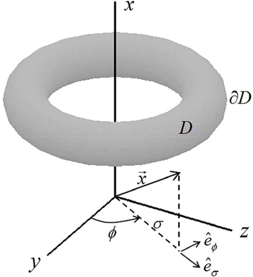
Core of vortex ring and cylindrical polar coordinates
For an axisymmetric flow, the Helmholtz vorticity equation can be expressed as follows (Batchelor, 1967):
Based on Eq. (3), vorticity ωϕ is proportional to σ inside the core, and it is expressed in the equation below. Whereas it is an irrotational flow outside the core.
, where ∂D denotes the core boundary, and Ω is a constant. The aforementioned formulation is also reported in Choi (2020).
The fluid velocity vector u⃗ can be calculated using the Green’s 2nd identiy (Shariff et al., 1989; Shariff et al., 2008) as follows:
However, the curl of vorticity vector in Eq. (5) exhibits the following behavior due to the jump in vorticity across the core boundary ∂D in Eq. (4).
Therefore, u⃗ in Eq. (5) can be expressed as the sum of the integrated value inside the core u⃗C and integrated value in the small region crossing the boundary u⃗J as follows:
According to Shariff et al. (1989) and Shariff et al.(2008), u⃗C and u⃗J are determined based on the following equations, which are expressed as contour integrals.
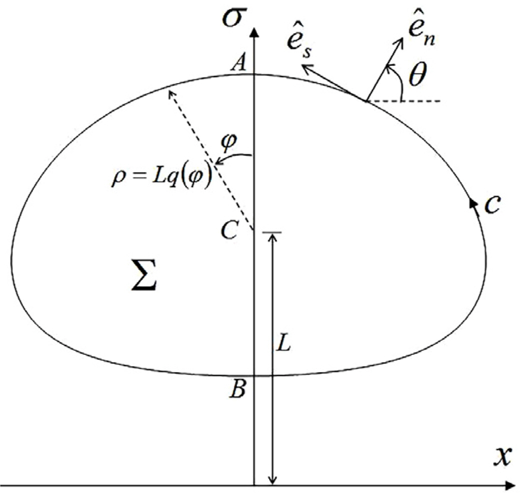
Meridional cross section of the core of vortex ring
When (x, σ)∈c in Eqs. (13) and (14), the movement of a vortex ring can be analyzed. In this study, the N-F family of vortex rings, which are in a steady state, were analyzed. In this case, a vortex ring advances forward in the positive x-direction at a constant speed U. Given that the core boundary c exhibits the characteristics of a material boundary, it should satisfy the following impermeable boundary condition.
To define the size of a core, Norbury (1973) expressed the cross-sectional area AΣ of the core using the ring radius L in Fig. 2 and non-dimensionalized mean core radius α as follows:
Circulation (Γ), vortical impulse (Γ), and kinetic energy (T) of a inviscid vortex ring are invariant and expressed as follows (Lamb, 1932):
Furthermore, forward speed U can be derived by determining vorticity center (x̄Γ ) and impulse center (x̄P) using Eq. (17) and (18), respectively, and then taking their time derivatives (Lamb, 1932). By considering circulation and impulse as invariants and using the Reynolds transport theorem, U can be expressed as follows:
In this study, physical quantities were non-dimensionalized as the methods in studies by Norbury (1973) and Choi (2020).
Eqs. (13) and (14), which are fluid velocity components, can be non-dimensionalized as follows:
For expressing contour shapes, radius q(φ) from point C and the parameter angel φ are introduced as shown in Fig. 2 (Norbury, 1973; Choi, 2020).
Non-dimensionalized cross-sectional area of the core, circulation, and impulse are as follows (Choi, 2020):
For a given value of α, in this study, we aim to ensure that the fluid velocity components calculated from Eqs. (28) and (29) satisfy the boundary conditions in Eq. (15) and to find a contour shape whose cross-sectional area satisfies Eq. (31).
Pozrikidis (1986) demonstrated that kinetic energy in Eq. (19) can be calculated using line integral as shown below.
However, the stream function value satisfies the following relation on contour c (Norbury, 1973; Choi, 2020).
The kinetic energy was computed using a two-dimensional integral in Eq. (34) because the fluid velocity cannot be determined if the CD method for a stream function is used (Choi, 2020). By using the CD method for the fluid velocity proposed in this study, we can substantially reduce the number of computations because contour integral in Eq. (36) is used in computations.
U values deduced from vortical center and impulse center are as follows:
3. Numerical Analysis Method
Considering the shape symmetry, the shape is discretized using nodal points and segments, as shown in Fig. 3, to determine the contour shape (Choi, 2020).
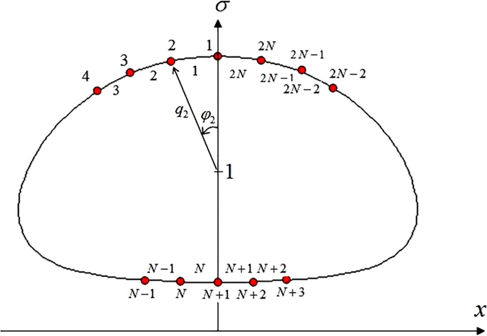
Discretization of contour (Choi, 2020)
Based on the definition of point C (Fig. 2) and symmetry, the following relations are established.
If N number of q1 to qN, which satisfy Eqs. (15) and (31), can be determined for given α, then the discretized shape of contour can be determined. Furthermore, the forward speed U is an unknown value that should be determined. Therefore, the total number of unknowns is N + 1. Given that Eq. (15) is automatically satisfied if the field point is (x1,σ1) or (xN+1,σN+ 1), the number of conditional equations that can be applied using this equation is N − 1. The following conditional equation determined from the relation between Eqs. (37) and (38) can be used; the total number of conditional equations is N + 1 when Eq. (31) is used, and therefore, N + 1 unknowns can be calculated.
To determine the solution for N + 1 nonlinear system of equations, an initial shape was assumed and an iterative method was applied (Choi, 2020). In this study, Broyden’s method was applied as the iterative method (Press et al., 1992). Furthermore, angle was divided into equal intervals.
Contour integrals in Eq. (28) and Eq. (29) are summed as segment integrals as follows:
where lx=xi+1−xi, lσ=σi+1−σi, 0 ≤ ξ ≤ 1
Eq. (46) can be substituted into Eqs. (44) and (45) as follows:
When n≠i and n≠(i+1), general numerical integrals can be considered because integrands of Eqs. (47) and (48) show a non-singular behavior. In this study, numerical integrals were performed using three-point Gauss–Legendre quadrature (Choi, 2020).
However, when n = i or n =(i+1), integrals should be performed by considering logarithmic singularity generated when ξ = 0 or ξ = 1, respectively. When n = i, Eqs. (47) and (48) are expressed as follows.
Based on the methods proposed by Shariff et al. (1989), Shariff et al. (2008), and Choi (2020), H and G were asymptotically expanded at ξ = 0 to take integrals analytically.
In Eq. (51), the integration values calculated by setting JM = 5 are presented in Appendix. When δux,n(xn +1,σn+1) and δuσ,n(xn+1,σn+1), the signs of lx and lσ are reversed in Eqs. (49)–(50) and Eqs. (A1)–(A3); when σn+1 is used instead of σn, the signs of the integrals are reversed.
A derivative of a contour curve is required to find cosθ and sinθ, which are the components of a normal vector in the boundary condition of Eq. (15).
A Fourier cosine series was used in this study to determine the slope of a continuous contour curve from the discretized contour shape.
The solution does not converge or cannot be determined even when numerical differentiation was performed by using the nearby nodal points or derivatives of a cubic spline curve to determine the derivative of the contour curve.
4. Analysis Results
The initial guess for the iterative method was set similar to the method in a study by Choi (2020). When α≤0.95, a circle with a radius of α was set as the initial guess for counter; for 0.95 <α≤1.0, a circle with the radius of 0.95 was used as the initial guess for contour. Here, the initial guess of U was set to 0.5. When α >1.0, the solution for α = 1.0, 1.1, 1.2, 1.3, 1.39 was sequentially calculated to set the initial guess value.
The number of segments used for the analysis was set identical to that in the study by Choi (2020), or 2N = 120.
The core shape of several α values is illustrated in Fig. 4. An interpolated value based on the Fourier analysis was used for the shape between nodal points. Specifically, half of the results of this study and those of the study by Choi (2020) were illustrated considering symmetry. The core shape was almost identical to the result in the study by Choi (2020), in which the CD method for a stream function was used. Thus, using the CD method for the fluid velocity is also appropriate for analyzing the vortex ring in a steady state. Furthermore, the excellence of the CD method based on the direct method is exhibited when compared to the results of the study by Norbury (1973) (Choi, 2020).
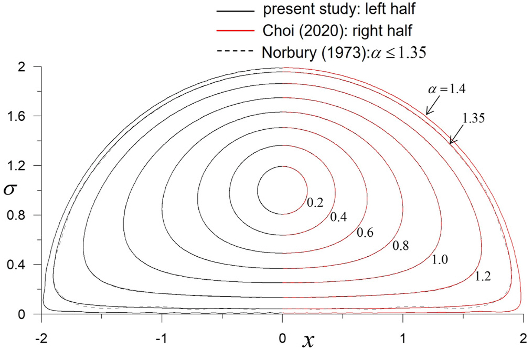
Contour shapes for various values of α
Shariff et al. (1989) and Shariff et al. (2008) conducted a dynamic analysis by applying the shape results of Norbury (1973) as the initial condition when α = 0.6 to verify the convergence of the dynamic analysis results based on the number of segments. Regarding the analysis results based on 200, 400, 800, and 1,200 segments, the shape of a steady state was maintained even after time had passed when the number of segments was 1,200. Conversely, in this study, an analytical method was proposed to determine the shape of the N-F family vortex ring via iterative methods based on the initially estimated shape, and the results were superior to those reported by Norbury (1973).
If only computation convenience is considered, the method proposed by Choi (2020), which uses a stream function to directly express shapes, is superior than the method proposed in present study, which estimates shapes based on two velocity components and shape slope. However, the CD method for fluid velocity should be introduced to expand the proposed method for an unsteady fluid analysis.
Fig. 5 illustrates the analysis results for forward speed U, κ in Eq. (35), and the core volume VΣ. Furthermore, constant κ was determined at each nodal point by applying the deduced contour to the method proposed by Choi (2020). The constant value must be identical in principle, but a small numerical error is observed at each nodal point. In this study, an arithmetic mean of κ of each nodal point is used. The results of this study correspond to those of the studies by Choi (2020) and Norbury (1973), in which stream functions were used.

Translation velocity (U), κ, and core volume (VΣ)
The analysis results of circulation, vortical impulse, and kinetic energy are illustrated in Fig. 6. Given that Norbury (1973) and Choi (2020) only used stream functions when calculating kinetic energy, a two-dimensional integral in Eq. (34) should be performed. However, the number of computations can be drastically reduced because kinetic energy is calculated using the line integral of Eq. (36) based on the fluid velocity. The kinetic energy result obtained in this study corresponds to the result obtained by Choi (2020), but the values are slightly greater than the result reported by Norbury (1973).
Circulation (Γ), vortical impulse (P), and kinetic energy (T)
5. Conclusion
In this study, we examined whether the CD method for fluid velocity, which is used for dynamic analysis, can also be applied for the analysis of a vortex ring in a steady state. When compared to conventional analysis results based on the Stokes’ stream function, the CD method for fluid velocity is applicable for analyzing the N-F family of vortex rings.
The speed of the vortical center and impulse center corresponds to the forward speed of a vortex ring, and the solution can be obtained by additionally applying a conditional equation, which sets the two speeds as identical. A normal vector can be obtained at the discretized nodal point of a shape via Fourier analysis. The normal vector was eventually used to determine the converged iterative calculation results. The degree of numerical integration was heightened by analytically performing the integral of logarithmic singularity.
In future studies, the stability of the N-F family of vortex rings due to a small disturbance can be examined based on the proposed method.
Notes
No potential conflict of interest relevant to this article was reported.
References
Appendices
Appendix
The integral values at the logarithmic-singular segment based on the asymptotic expansion of Eq. (51) are expressed as follows.