Single Image-based Enhancement Techniques for Underwater Optical Imaging
Article information

Abstract
Underwater color images suffer from low visibility and color cast effects caused by light attenuation by water and floating particles. This study applied single image enhancement techniques to enhance the quality of underwater images and compared their performance with real underwater images taken in Korean waters. Dark channel prior (DCP), gradient transform, image fusion, and generative adversarial networks (GAN), such as cycleGAN and underwater GAN (UGAN), were considered for single image enhancement. Their performance was evaluated in terms of underwater image quality measure, underwater color image quality evaluation, gray-world assumption, and blur metric. The DCP saturated the underwater images to a specific greenish or bluish color tone and reduced the brightness of the background signal. The gradient transform method with two transmission maps were sensitive to the light source and highlighted the region exposed to light. Although image fusion enabled reasonable color correction, the object details were lost due to the last fusion step. CycleGAN corrected overall color tone relatively well but generated artifacts in the background. UGAN showed good visual quality and obtained the highest scores against all figures of merit (FOMs) by compensating for the colors and visibility compared to the other single enhancement methods.
1. Introduction
Optical images generated by the reflected light from an object are useful and intuitive for visual monitoring in unknown underwater environments. On the other hand, reflected light is typically scattered and absorbed by water and floating particles. This light attenuation causes low visibility with haziness and color cast in the resulting optical image (Mobley, 1994). The color cast effect produces a greenish or bluish hue in underwater optical images due to different attenuations depending on the light wavelength. Red light is attenuated more than green and blue light because of its longer wavelength. Depending on the transmission distance, water attenuation can cause limited visibility due to the loss of light intensity and contrast.
Considerable efforts have been made to compensate for the limited visibility and color cast effect of underwater optical images. The focus of most studies is on estimating a distance map because light attenuation of a specific wavelength is dependent on the distance from the camera. Stereo imaging has been used in some studies to obtain a distance map or enhance image quality directly (Roser et al., 2014; Zhang et al., 2014). Stereo imaging has been used to recover underwater images through a physical image formation model and an estimated distance map. One other approach has enhanced the underwater image by utilizing multi-directional light sources and fusing these different light images (Treibitz and Schechner, 2012). This study focused solely on single image enhancement as opposed to multi-images. This is because the utilization of multi-image enhancements requires additional hardware devices that are not available as a general imaging platform in the context of an underwater environment.
Single image enhancement improves image quality using the information extracted from a given underwater image. A single image enhancement technique is to adopt prior physical knowledge of light. Dark channel prior (DCP) is popular and was proposed to improve the haze of outdoor images using a light transmission map estimated from the darkest color channel (He et al., 2011). DCP has been applied widely to remove the turbidity of underwater images. On the other hand, it is imperfect for estimating a light transmission map due to nearly zero red channel values in the underwater environment. Underwater DCP estimates light transmission, excluding the red channel (Drews et al., 2013). For single image enhancement, the maximum intensity prior calculates the difference between the maximum values of red, green, and blue channels to estimate the light transmission map (Carlevaris-Bianco et al., 2010).
Domain transform methods were applied to single image enhancement. A homomorphic filter was used to help suppress noise and amplify details in the image frequency domain (Luo et al., 2019). The wavelet transform has been used for denoising (Jian and Wen, 2017) or fusing images (Khan et al., 2016; Wang et al., 2017a). The gradient-domain transform method has been found to recover the original gradient instead of the image intensity itself based on the image formation model (Li et al., 2012; Mi et al., 2016; Park and Sim, 2017; Zetian et al., 2018). Typical image processing techniques have been applied for contrast and turbidity enhancements. Multiple image processing steps have been established to improve the contrast, noise, and color successively (Arnold-Bos et al., 2005; Bazeille et al., 2006; Ghani and Isa, 2014; Ghani and Isa, 2015). The image fusion method was also proposed to combine the characteristics enhanced in multiple image processing steps (Ancuti et al., 2017). The combined technique of domain transform and fusion was proposed to dehaze general color images in air (Cho et al., 2018).
Recent research has found that deep neural networks for underwater optical imaging can enhance underwater images directly (Anwar et al., 2018; Fabbri et al., 2018; Guo et al., 2019; Hou et al., 2018; Li et al., 2019a; Li et al., 2019b; Sun et al., 2018; Uplavikar et al., 2019; Wang et al., 2017b) or estimate inherent information, such as background light intensity and transmission maps (Cao et al., 2018; Li et al., 2018a; Li et al., 2018b). Training convolutional neural networks require huge pairs of underwater images and clean images, but clean images are difficult to obtain in an underwater environment. Therefore, some researchers have used indoor datasets of color images and the corresponding depth information (Anwar et al., 2018; Cao et al., 2018; Hou et al., 2018; Uplavikar et al., 2019) or applied unsupervised networks, such as a generative adversarial network (GAN), to produce the image pairs (Fabbri et al., 2018; Guo et al., 2019; Li et al., 2019b). A detailed review of underwater image enhancement techniques can be found elsewhere (Anwar and Li, 2019; Wang et al., 2019; Yang et al., 2019).
In this study, six single image enhancement methods were considered: original DCP, gradient transform method with Tarel’s and Peng’s transmission maps, image fusion of successive three image processing steps, and two GANs. Although original DCP and Tarel’s methods were designed to enhance the haze outdoor environments, they were applied to underwater images because underwater images suffer from haziness. The gradient-domain transform was selected from the domain transform methods available because it simplifies the image formation model, and two different methods proposed by Tarel and Hautière (2009) and Peng and Cosman (2017) were applied to estimate a transmission map. Peng and Cosman (2017). proposed specific ways to estimate a depth map and background lights considering the underwater environments. The image fusion method should be an effective way to improve by combining appropriate image processing techniques. Two GANs, CycleGAN and underwater GAN, which are designed for underwater image enhancement, were applied because GAN is a new remarkable deep learning algorithm for various applications of image processing. The enhancement performance was assessed quantitatively in terms of underwater image quality measure (UIQM) considering the colorfulness, sharpness, and contrast, underwater color image quality evaluation (UCIQE) considering color saturation, chroma, and contrast and gray world (GW) assumption as color correction metrics, and blur metric. The comparison results would help other researchers better understand the advantages and disadvantages of single image enhancement methods for their studies.
This paper is organized as follows. Section 2 describes the single image enhancement methods considered in this study. Qualitative and quantitative comparisons are reported in Section 3. Sections 4 and 5 discuss the results and outline the conclusions of this study.
2. Single Image Enhancement
The light transmitted through water can be defined by the simple image formation model as follows (Fattal, 2008):
2.1 Dark Channel Prior Enhancement
He et al. (2011) reported that at least one of the R, G, B-color channels in a pixel tends to approach zero in a colorful image. They proposed DCP to estimate the transmission from the darkest color channel in a local patch of given observed light, I. The dark channel image, Jdark, of a clean original image can be defined by the minimum operator (min[ ]) over a local patch and three color channels. This will approach zero according to DCP as follows:
2.2 Gradient Transform Enhancement
The gradient transform method was derived by adopting a gradient of Eq. (1) (Li et al., 2012). Assuming that the transmission is constant in a local patch, the gradient of I may be represented simply as follows:
The gradient transform method estimates the transmission for obtaining the original image gradient, ∇J, from a given ∇I. The enhanced original image, J̃, was then reconstructed from its gradient, ∇J, via the Poisson equation solver assuming Dirichlet boundary conditions. Based on the calculus of variations, the cost function can be defined using Eq. (6) to recover the image intensity from its gradient:
The Euler-Lagrange equation was adopted to minimize the integral of F( ) in (6) and the Poisson equation in Eq. (8) was then derived from Eq. (7):
Here, ∇2 is Laplacian operator, and div is the divergence operator. Using the Dirichlet boundary condition, a boundary image, B of J̃ was defined as containing all zero pixel values, except for the boundary pixels of J̃. Table 1 lists the estimated final recovered image, J̃, from the Poisson equation (Simchony et al., 1990).

Image reconstruction from a given gradient
This paper considered two transmission estimation methods. Tarel and Hautière (2009) proposed patch-based processing, such as DCP, and adopted the Median operator Along Lines (MAL). This preserves the edges without the halo effect as well as the corners, unlike the classical median operator, as shown in Eq. (9):
Ω(x) was defined as the line segments over a square patch centered at x. Each line segment must pass through the center of the square patch. The MAL performs a classical median filter along each line segment and then calculates the median of the median values of each line segment. The number of line segments and the patch size are key parameters determining the enhancement performance. This study set five line segments and a 61×61 patch size.
Peng and Cosman (2017) estimated the transmission from a depth map based on image blurriness and light absorption by water and floating particles and the attenuation coefficients (μc) corresponding to RGB colors, as follows:
The depth map, d(x) can be calculated with two relative depth estimates, d0 and dmix . This is based on different light absorption phenomena of RGB colors and the mixed additional distance information relative to the closest distance as follows:
dmix was determined using three depth-related values accommodating the different attenuations of RGB color signals and blurriness of the underwater image, as follows:
The mixing weights, α and β were determined from the average intensities of background light and the red channel in the input image as follows:
The local patch size was set to 5×5 in max[ ] operator. fN[ ] normalizes the input value in the range of 0 to 1. dblur is estimated by the blurriness in the underwater image as follows:
Blurriness was defined by the mean of edge information extracted at various Gaussian kernel sizes, as follows:
Igray is a gray-scaled image of the underwater color image. Gauss is a Gaussian filter with a kernel size, σ of 2lL+1 at different kernel levels, {l = 1, ⋯, L}. L was set to 4. Fill[ ] operator performs a morphological opening to compensate for the sparse regions and holes in Iblur to become denser (Vincent, 1993). Calculation of background light intensity is required to determine the closest distance and the mixing weights. The background light intensity was determined by combining the maximum and minimum of the three background light components,
First, the transmission of the red channel, tr, was determined using the estimated distance map in Eq. (11), background light in Eq. (19), and the attenuation coefficient, μr, was set to 1/7 for Ocean Type-I water (Zhao et al., 2015). The attenuation coefficient ratios between the red and other colors were used for transmission conversion from red to blue and green colors as follows:
The wavelengths, λc of the red, green and blue colors are 620, 540, and 450 nm, respectively.
2.3 Image Fusion Enhancement
Image fusion enhances features in an image and fuses the enhanced images (Ancuti et al., 2017). This consists of three processing steps: white balancing, feature enhancing, and image fusing. In the image fusion method, white balancing compensates the red and blue signals giving them flatter distributions compared to the green signal, which tends to maintain its intensity through water somewhat.
After white balancing to correct for color casting by water, two feature enhancing techniques were applied independently. First, contrast-limited adaptive histogram equalization (CLAHE) was adopted instead of gamma correction in the original method to enhance image contrast (Icontrast). CLAHE performs an ordinary histogram equalization over the predefined patch with a limited clip level. The parameters of CLAHE are the patch size, Ω, and a histogram clip level, hl. Furthermore, unsharp masking was applied to sharpen features, such as an edge in an image, as follows:
Three weight maps of Laplacian contrast, saturation, and saliency were determined to fuse two images enhanced from the previous step. The Laplacian contrast weight map, ωLap, depends on global contrast in an image and was calculated as the absolute value of the Laplacian filtered luminance signal of each enhanced image, as follows:
The saliency weight map, ωSal, represents the prominent features of an image in CIELAB color space (Achantay et al. 2009), and can be expressed using Eq. (26):
The Gaussian kernel size was set to 3×3. The final weight map for each enhanced image from the previous step, combined three weight maps with normalization, as follows:
The Laplacian pyramid at each lth level quantifies the difference between an input image and its Gaussian filtered image after sampling-down the operation by a factor of 2. The size of the Gaussian kernel in the pyramid computation was set to 5×5. The number of pyramid levels, pl, was set to 3.
2.4 Generative Adversarial Network Enhancement
A convolutional neural network is a widely used deep learning network for many image processing applications. Robust training in a deep learning network requires huge datasets and a reliable ground truth. On the other hand, it is difficult to construct ground truth for underwater color images. Fabbri et al. (2018) proposed underwater GAN (UGAN) to increase the reliability of synthetic training data and enhance underwater color imagery using synthetic data. GAN typically consists of the generator and discriminator networks, and the training process is performed by optimizing the loss function in Eq. (29):
The generator network (G) competes against discriminator (D) during training to generate exquisite fake images and deceive the discriminator. The discriminator is trained to distinguish a fake image from a generator. The loss function of UGAN was defined with the Wasserstein GAN loss function and gradient penalties.
Wasserstein loss function, ℒWGAN, was proposed to solve the training issue induced by the general GAN loss function, which measures a difference between real and generated data distributions in Eq. (29) (Arjovsky et al., 2017). ℒWGAN is expressed as follows:
The weight, η0 was set to 10. ℒL1 is defined by the L1-norm of the difference between the ground truth and the image predicted, JP, by the generator, as follows:
The hyper-parameters, η1 and η2 were set to 100 and 1, respectively.
Fig. 1 summarizes the architecture of the discriminator and generator networks of UGAN. The discriminator network adopted the PatchGAN model (Isola et al., 2017) that was comprised of five convolutional layers, and the resulting output feature map was 32×32. Each convolutional layer of the PatchGAN model performs the convolution operation, followed by ReLU activation. The generator has a U-Net model consisting of encoder and decoder sections in a U-shape (Ronneberger et al., 2015). The encoder and decoder sections in U-Net have eight convolutional and seven deconvolutional layers, respectively. Each convolutional layer of the U-Net model performs successive convolutions with a 4×4 kernel and stride of 2, batch normalization, and leaky ReLU activation. The deconvolution layer also includes a 4×4 convolution kernel with a stride of 2 and ReLU activation, without batch normalization. The outputs from the second to seventh convolutional layers were connected to the outputs of deconvolutional layers in U-Net. UGAN was trained with the paired synthetic datasets of underwater and clean ground truth images. To construct the paired datasets, an unsupervised network, cycleGAN, was applied to a mapping function of clean to underwater images: F: J→I (Zhu et al., 2018). CycleGAN consists of a Resnet-9 block generator and a PatchGAN discriminator outputting a 70×70 feature map. CycleGAN was trained with two batches and 100 epochs using 6,050 clean images and 5,202 underwater images. This included 1,813 images from ImageNet (Deng et al., 2009) and 3,389 real images taken in Korean waters. The trained cycleGAN generated pairs of clean and underwater images where 5,202 underwater images were used for training. From the paired training images, UGAN was trained with 32 batches and 20 epochs.
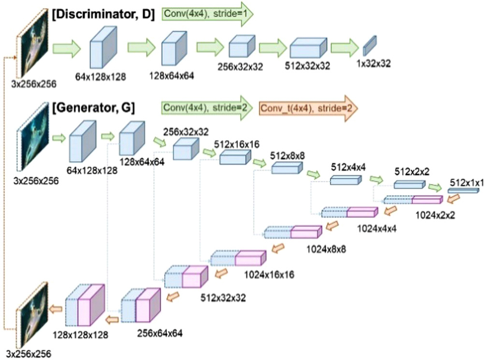
UGAN network architecture: The generator transforms an underwater image into a fake clean image through a u-shape network consisting of an encoder and decoder. The discriminator takes the generated image as input and produces a 32×32 patch image to distinguish between the real clean image and the fake clean image.
3. Results
The performances of the DCP, two gradient transform methods, image fusion, cycleGAN, and UGAN were compared by evaluating the image quality of real underwater images taken in Korean waters. The enhancement was evaluated quantitatively based on UIQM, UCIQE, GW assumption, and blur metric.
UIQM was calculated using the weighted sum of colorfulness (UICM), sharpness (UISM), and contrast (UIConM) measures (Panetta et al., 2016). This study used the same weighting as Panetta et al. (2016); a1= 0.0282, a2= 0.2983, and a3= 0.0339. The computation of UIQM is expressed in Eq. (34):
UICM was measured by the mean and standard deviation in two combined color domains of the image to be evaluated; red-green and yellow-blue colors, as follows:
In the combined color domains, Irg = Ir − Ig and Iyb = (Ir − Ig)/2− Ib. μα and σρ are the mean and standard deviation of Irg and Iyb. ρ is a ratio to trim the upper and lower intensity pixels. The UISM sharpness was evaluated based on the weighted sum of the difference between the maximum and minimum values in the edge map for each color channel, as shown in Eq. (36). The edge map was determined by the Sobel operator as follows:
UCIQE is calculated by a weighted sum of three measures in terms of the chroma (σchr ) and luminance (conLum ) in CIELAB color space and saturation (μsat) (Yang and Sowmya 2015), as expressed in Eq.(39):
In CIELAB color space, [L,a,b] of an image, the standard deviation of chroma (σchr ) was calculated by
The GW assumption is that an equal mixture of RGB color channels should be neutral gray under a color-balanced situation. An underwater GW assumption was used to measure the degree of color correction (Berman et al., 2018). Here, the calculation process for the GW value was modified with a standard deviation over three mean color values. The color balance improves as the GW becomes lower, as follows:
The blur metric is derived based on observing that humans find it difficult to perceive differences between a blurred and re-blurred image (Crété-Roffet et al., 2007). The blur measure compares the horizontal and vertical derivatives of an input and its blurred images by the max operator. Blur metric was normalized from 0 to 1; a larger blur metric value indicated more blurring.
Directional sum, difference, and derivative operators were applied to input (I) and its blurred images (Ib = blur[IY]) in the luminance channel according to Eqs. (42) and (43). The blur[ ] operator averaged nine elements horizontally and vertically.
If the input image already has high blurriness, the difference between the directional derivatives of the input and blurred image would be small, resulting in a larger blur metric value.
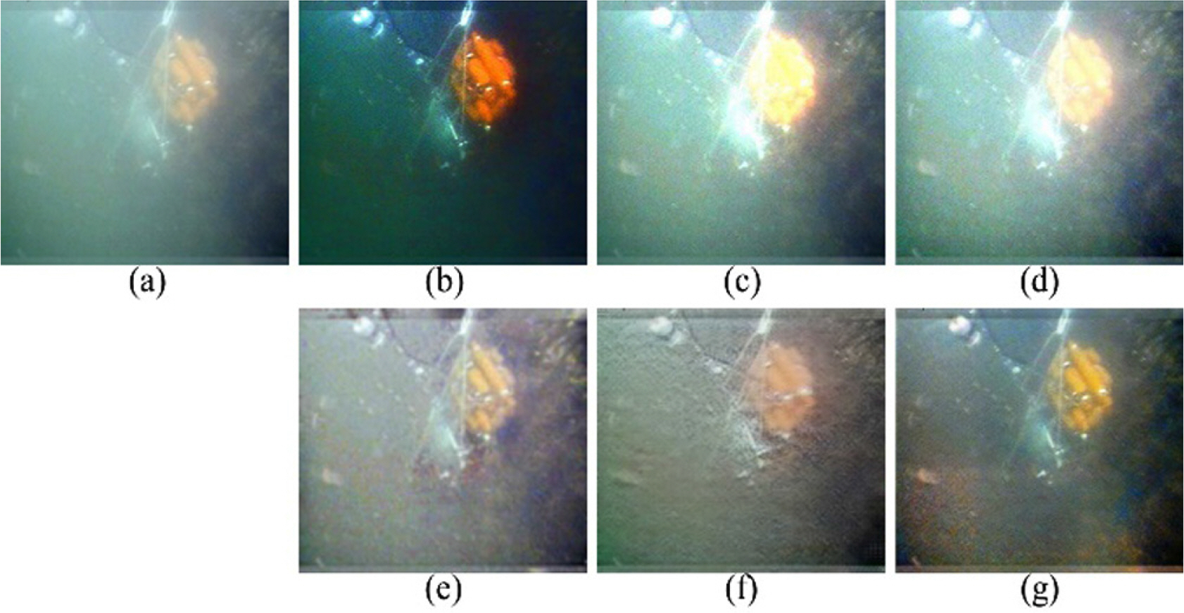
Figs. 2 to 4 present images enhanced using single enhancement methods from real underwater images. Three underwater images were captured with a dominant greenish color tone and exposure to a strong light source from standard definition (SD) videos recorded in the late afternoon. Figs. 2 and 3 were taken in May 2015 at Jangmok Port, Geoje-si, Gyeongsangnam-do using a camera equipped with a Pro 4 ROV (VideoRay, USA). Fig. 4 was recorded in November 2017 at Yokjido, Tongyeong-si, Gyeongsangnam-do, using an SD camera equipped with a BlueROV (BlueRobotics, USA). All scenes were illuminated by LED lighting equipped in the ROVs. DCP, (b) in Figs. 2 to 4, tends to emphasize a green color in the overall scene and darkens the background signal. DCP was ineffective in correcting the greenish color cast effect, which is the main artifact of underwater imagery. Gradient transform with Tarel and Peng transmissions were sensitive to the brightness change in an underwater image, as shown in (c) and (d) of Figs. 2–3. This was also found to be ineffective in enhancing the object details, as illustrated in Figs. 4(c) and (d). Two gradient-Tarel and Peng inadequately corrected for the overall greenish color tone in all underwater images. Image fusion moderately compensated for the overall color tones in (e) of Figs. 2 to 4. On the other hand, it did not enhance the image contrast of objects or reduce the haziness in the background. CycleGAN provided good correction of the overall colors and enhanced the object details, but it generated artifacts in the background, as shown around objects in Fig. 3(f). UGAN provided good visual quality in terms of compensating for the greenish color tone, enhancing the object details, and reducing haziness comparing to the other enhancement methods in (g) of Figs. 2 to 4.

(a) Real original underwater image of 481×416, showing a dominant greenish color tone and exposure to strong light at the top, and the enhanced images by (b) DCP, (c) gradient-Tarel, (d) gradient-Peng, (e) image fusion, (f) cycleGAN, and (g) UGAN.

(a) Real original underwater image of 711×406, showing low contrast and visibility, and the enhanced images by (b) DCP, (c) Gradient-Tarel, (d) Gradient-Peng, (e) Image fusion, (f) CycleGAN, and (g) UGAN.
(a) Real original underwater image of 481×416, showing a dominant greenish color tone and expose to strong light in the middle, and the enhanced images by (b) DCP, (c) gradient-Tarel, (d) gradient-Peng, (e) image fusion, (f) cycleGAN, and (g) UGAN.
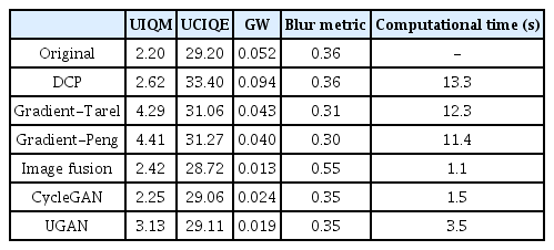
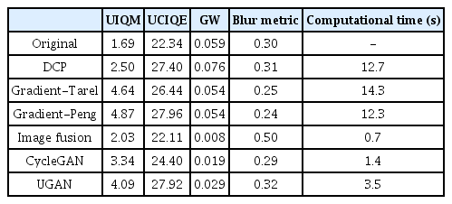
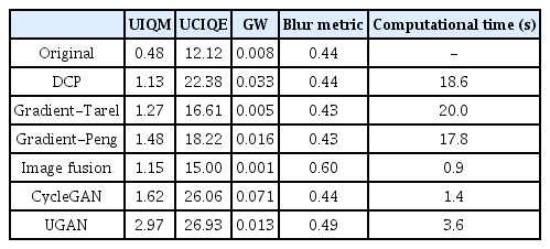
Tables 2 to 4 compare the figures of merit (FOM), i.e., UIQM, UCIQE, GW, blur metric, and computational time, evaluated from the original and the enhanced underwater images in Figs. 2 to 4. UIQM and UCIQE were difficult to interpret because they focus on different aspects depending on the example image. Unlike a visual comparison, two gradient transform methods and DCP obtained a high UIQM and UCIQE for Figs. 2 and 3. For all underwater images, DCP obtained the highest UCIQEs for Figs. 2 and 3 because of high color scores with respect to σchr, and μsat. This might be due to DCP’s tendency to increase the saturation of underwater images for a specific color. Gradient transform methods tended to emphasize the bright region exposed to light, which increases the sharpness and contrast score. Thus, two gradient transform methods had the highest UIQM and UCIQE because of the high sharpness (UISM) and contrast (conLum) measures, respectively. Image fusion had the best and the worst scores in terms of the GW color quality and blur metrics, respectively. This shows that image fusion is effective in balancing underwater colors, but makes the images blurry. CycleGAN and UGAN showed high UIQM and UCIQE in all figures. Furthermore, the two GANs had better GW scores than the original underwater images and the same blur scores as the original image for Figs. 2 and 3. Marginal differences were observed between the two GANs in terms of all FOMs for Figs. 2 and 3. In terms of Fig. 4, UGAN had higher UIQM and GW scores than cycleGAN. The computational time associated with each enhancement method was compared on an Intel Core i7-7700HQ CPU. The training time of cycleGAN and UGAN are approximately 46 hours and 12 hours on a Nvidia Quadro P4000 GPU, respectively. The two GANs ran on Python with the Tensorflow framework. The other methods ran on MATLAB. Image fusion and two GANs had the best and moderate computational time performance, respectively, compared to the other single enhancement methods.
4. Discussion
This study applied single image enhancement approaches, DCP, gradient transform method with Tarel and Peng transmission maps, image fusion, and two GANs of cycleGAN and UGAN, to compensate for the color cast effect and low visibility due to the light attenuation underwater. The enhanced performance was evaluated in terms of UIQM, UCIQE, GW, and blur metrics with real underwater images taken in Korean waters.
The original DCP was proposed to improve the hazy outdoor images by saturating the inherent color in a haze-free image. Saturation with a specific color produced strong greenish or bluish hues on the underwater image; both are already dominant color tones in underwater images. In DCP, the user needs to adjust the patch size of the min operator in Eq. (3). The DCP result was evaluated with different patch sizes of 11×11 to 21×21 with intervals of 2; however, there were no different effects on color correction depending on patch sizes.
The gradient transform method recovers the underwater image from its gradient enhanced with an estimated transmission map and the gradient of the given input image. The gradient transform method with Tarel and Peng transmissions produced bright regions that appear as though they are exposed to strong light in Figs. 2 and 3. This method was also ineffective in reducing the color-cast effect and low visibility of underwater images. The adjustable parameters in the Tarel transmission estimation are the number of line segments and a patch size in Eq. (9). Successive numbers of line segments from 3 to 8 and different patch sizes from 41×41 to 101×101 in intervals of 20 were applied. On the other hand, there were no significant differences between the final enhanced images with different adjustable parameters. An estimation of Peng transmission can depend on the patch size for depth-related values in Eqs. (15) and (16) and the number of Gaussian kernel levels in Eq. (18). This study examined the dependency on different patch sizes from 5 to 17 in intervals of 3 and found little dependency on the patch size.
Image fusion had the worst blur scores in Figs. 2 to 4 and resulted in a loss of object detail. It contained a contrast enhancement step, which was replaced with CLAHE instead of gamma correction. The blurry results were attributed to the last fusion step, with multiple levels of Laplacian and Gaussian pyramids. When more than three levels of pyramids were set, the final result increased the blurriness. In contrast, small pyramid level numbers resulted in noisier images.
If naïve fusion is performed, as per Eq. (44), there is an increase in the sharpness of underwater images compared to multiscale fusion, but it produces random pattern artifacts in the background.
GAN might be affected by the generality of the training data to express underwater color images. Training data were constructed with ImageNet and real underwater images taken in Korean waters to identify the turbidity and color cast. The inclusion of real underwater imagery in Korean waters improved the color tone and visibility compared to the training data in the ImageNet database. The pre-trained cycleGAN was applied to improve underwater image quality and generate underwater and clean image pairs for training UGAN. CycleGAN and UGAN were compared to confirm the performances of unsupervised and supervised learning for single image enhancement because they do not require additional data, such as a depth map for training. CycleGAN had incomplete enhancement performance producing artifacts in the background. UGAN acted moderately to enhance the color balance and visibility of underwater images compared to the other enhancement methods, but it was not effective in dehazing the underwater images. To enhance visibility, a new network architecture needs to be constructed and trained with the paired underwater images and additional information like depth maps (Li et al., 2018b).
UIQM and UCIQE are popular FOMs used in studies of underwater enhancement. The method to combine three quality measures in UIQM and UCIQE is dependent on the weights in Eqs. (34) and (39). On the other hand, there were no proposed ways to determine the weights properly. In this study, it was difficult to interpret the general tendencies of UIQM and UCIQE because these FOMs fluctuated in each case by case, and the quantitative interpretations based on the scores were different from the visual comparisons. It is necessary to normalize the individual image quality measure of UIQM and UCIQE and to set reasonable weights to evaluate the overall image quality adequately. The GW assumption and blur metric were adopted to evaluate color balancing and blurriness in the enhanced underwater image. Individual FOMs, such as GW and blur metrics, reflected the consistent quantitative image quality measures compared to the combined FOMs of UIQM and UCIQE for underwater images.
5. Conclusions
In this study, six single underwater image enhancement approaches were compared: DCP, two gradient transforms, image fusion, and two GANs. The enhancement performances were evaluated qualitatively and quantitatively. DCP caused saturation of the underwater images to either a greenish or bluish color tone and reduced the brightness of the background signal. The gradient transform methods with two transmission maps were sensitive to the light source and highlighted the region exposed to light. Image fusion provided reasonable color correction, but the object details were lost due to the last fusion step. CycleGAN corrected the overall color tone well, but generated artifacts in the background. Although UGAN was not rated with the best scores for three sample images, it showed fairly good visual quality and quantitative scores for all FOMs.
Acknowledgements
This study was supported in part by research grants from Basic Science Research Program through the National Research Foundation of Korea (NRF) funded by the Ministry of Education (NRF- 2018R1D1A1B07049296), and by the project titled ‘Development of the support vessel and systems for the offshore field test and evaluation of offshore equipment’, funded by the Ministry of Oceans and Fisheries (MOF), Korea.