Energetics of In-plane Motions in Coupled Plate Structures

Young-Ho Park; Chang Hyun Park

doi:10.26748/KSOE.2020.063

Abstract

Energy flow analysis (EFA) has been used to predict the frequency-averaged vibrational responses of built-up structures at high frequencies. In this study, the frequency-averaged exact energetics of the in-plane motions of the plate were derived for the first time by solving coupled partial differential equations. To verify the EFA for the in-plane waves of the plate, numerical analyses were performed on various coupled plate structures. The prediction results of the EFA for coupled plate structures were shown to be accurate approximations of the frequency-averaged exact energetics, which were obtained from classical displacement solutions. The accuracy of the results predicted via the EFA increased with an increase in the modal density, regardless of various structural parameters. Therefore, EFA is an effective technique for predicting the frequency-averaged vibrational responses of built-up structures in the high frequency range.

Nomenclature

<e>: Energy density (J/m2)

cg: Group velocity (m/s)

ω: Angular frequency (rad/s)

k: Wave number (rad/m)

q: Intensity (J/m/s)

1. Introduction

The demand for ecofriendly and lightweight systems has been gradually increasing in the transport machinery industries, e.g., shipbuilding, automobiles, aviation, and railroads, with the growing interest in environmental issues caused by global warming and the development of industrial technology. These industrial changes have increased the proportion of vibration noise in the high frequency range, exacerbating the vibration-noise issue of transportation machinery systems. Therefore, developing technology for predicting the vibration noise in the corresponding frequency range is becoming important for ensuring competitiveness in the transport machinery industries. Typically, deterministic approaches based on displacement methods, such as the conventional finite element method and boundary element method, have been utilized for vibration noise prediction method in the low frequency range. However, because these methods lack efficiency and reliability, statistical approaches such as statistical energy analysis (SEA) and energy flow analysis (EFA) are generally applied in the high frequency range. Numerical methods such as the finite element technique can be applied in EFA because it has an energy governing equation in the form of a differential equation, in contrast to SEA. Thus, EFA has recently emerged as a new alternative to high-frequency range vibration noise analysis, because the modeling efficiency is high and a detailed design review of the design parameters can be performed. In the early days after EFA was proposed by Belov et al. (1977), an energy flow model for out-of-plane motion was developed, which was mainly based on various simple structural element theories, e.g., those of the membrane, Euler beam, and Kirchhoff plate. Recently, however, Park and Hong (2006a), Park and Hong (2006b), and Park and Hong (2008) developed an energy flow model of the Timoshenko beam and Mindlin plate that reflects the shear-deformation effect and rotatory-inertia effect to increase the accuracy of the previously developed EFA model in the high frequency range, thereby expanding the analysis area. When beams or plates are coupled at arbitrary angles in actual structures, such as ships and offshore structures, the out-of-plane motion and in-plane motion are coupled, and the modal density of the in-plane motion increases with the frequency, increasing the importance of the model for in-plane motion in EFA. Therefore, Park et al. (2001) developed an energy flow model for in-plane motion for the EFA analysis of a coupled plate structure in a high frequency range. However, a study on the effectiveness of the energy flow model according to the frequency is needed, because no systematic comparison with the exact solution for the in-plane motion of the plate was performed in the study. In the present study, an exact solution of the in-plane motion for the plate coupled at an arbitrary angle was newly derived, and the effectiveness of the energy flow model for the in-plane motion of the plate was examined through comparison with the analysis results of the energy flow model.

2. Energy Flow Model for In-plane Motion of Plate

The equation of motion for the in-plane wave of a damped plate without a load can be expressed as follows (Dym and Shames, 2013):

(1)

∂2u∂x2+(1−ν)2∂2u∂y2+(1+ν)2∂2v∂x∂y=(1−ν2)ρEc∂2u∂t2

(2)

∂2v∂y2+(1−ν)2∂2v∂x2+(1+ν)2∂2u∂x∂y=(1−ν2)ρEc∂2v∂t2

where u and v represent the in-plane displacements of the plate in the x and y directions, respectively, E_c = E(1 + jη) represents the complex elastic modulus, η represents the structural damping loss factor, ν represents the Poisson’s ratio, and ρ represents the material density of the plate. The energy-flow model for the in-plane motion of the foregoing equation of motion can be derived by separating it into an in-plane longitudinal wave and an in-plane shear wave, as follows (Park et al., 2001):

(3)

−cg,l2ηω(∂2∂x2+∂2∂x2)〈el〉+ηω〈el〉=Πin,l

(4)

−cg,s2ηω(∂2∂x2+∂2∂x2)〈es〉+ηω〈es〉=Πin,s

where c_g_,_l and c_g_,_s represent the group velocities of the in-plane longitudinal wave and in-plane shear wave of a thin plate, respectively; 〈e_l〉 and 〈e_s〉 represent the energy densities of the in-plane longitudinal wave and in-plane shear wave averaged in space and time respectively; and Π_in_,_l and Π_in_,_s represent the vibrational input power for the in-plane longitudinal wave and in-plane shear wave, respectively.

3. Energy Flow Model for Out-of-plane Motion of Plate

The equation of motion for the out-of-plane motion of a damped Kirchhoff plate without a load can be expressed as follows (Dym and Shames, 2013):

(5)

Dc(∂2w∂x4+2∂4w∂x2∂y2+∂4w∂y4)+ρh∂2w∂t2=0

where D_c = D(1+jη) represents the complex flexural rigidity. The energy flow model for the flexural wave of the Kirchhoff plate derived from the foregoing equation of motion can be expressed as follows (Bouthier and Bernhard, 1995):

(6)

−cg,f2ηω(∂2∂x2+∂2∂x2)〈ef〉+ηω〈ef〉=Πin,f

where c_g_,_f represents the group velocity of the out-of-plane flexural wave of a thin plate, 〈e_f〉 represents the energy density of the out-of-plane flexural wave averaged in space and time and Π_in_,_f represents the vibrational input power of the out-of-plane flexural wave.

4. Analysis of Vibration Energy of Plate Coupled at Arbitrary Angle

The plate model coupled at an arbitrary angle was considered for an analytical study of the energy flow model for the in-plane wave of the plate.

4.1 Exact Solution of Coupled Plate Structures

In the exact solution of a coupled plate for which all the outer boundaries are simply supported, the displacement can be calculated in the form of a Levy series that satisfies the y-direction boundary condition equations, i.e., Eqs. (7)–(10). The displacement in the x- and y-directions in the i^th region can be expressed using Eqs. (11)–(13).

(7)

u1(0,y)=u3(Lx,y)=0

(8)

∂v1(0,y)∂x=∂v3(Lx,y)∂x=0

(9)

w1(0,y)=w3(Lx,y)=0

(10)

∂2w1(0,y)∂x2=∂2w3(Lx,y)∂x2=0

(11)

ui(xi,y,t)=[∑m=1∞Um,i(xi)sinkmy]ejωt

(12)

vi(xi,y,t)=[∑m=1∞Vm,i(xi)coskmy]ejωt

(13)

wi(xi,y,t)=[∑m=1∞Wm,i(xi)sinkmy]ejωt

Here, k_m = mπ/L_y and U_m_,_i(x_i), V_m_,_i(x_i), and W_m_,_i(x_i) represent the wave solutions in the x_i direction that satisfy the equation of motion. The following equation can be obtained by substituting the out-of-plane displacement expressed by Eq. (13) into Eq.(5), i.e., the equation of motion (Park et al., 2001).

(14)

d4Wm,i(xi)dxi4−2km2d2Wm,i(xi)dxi2+d4Wm,i(xi)dy4+(km4−kf4)Wm,i(xi)=0

Here, kf,i=(ρihiω2)/Dc,i4) represents the flexural wavenumber of the plate in the i^th plate section, and ρ_i and h_i represent the density and thickness of the plate, respectively. Because Eq. (14) is a fourth-order homogeneous ordinary differential equation, the wave solution of the displacement w in the x_i direction can be obtained as follows:

(15)

Wm,i(xi,t)=[Af1+exp(−αm,ixi)+Af1−exp(αm,ixi) +[Bf1+exp(−βm,ixi)+Bf1−exp(βm,ixi)]×ejωt

where αm,i2=km2+kf,i2 and βm,i2=km2+kf,i2. Although such an exact solution of the flexural wave, which is an out-of-plane displacement, was used to validate the energy flow model for the flexural wave of a plate, the exact solution of the in-plane displacement and the energy flow solution were not directly compared in previous studies (Park et al., 2001). Park and Hong (2008) derived an exact out-of-plane motion solution from the equation of motion implemented as the simultaneous differential equations for the Mindlin plate. The matrix equation can be obtained as follows by substituting Eqs. (11)–(12) into the simultaneous differential Eqs. (1)–(2) to obtain the wave solution in the x_i direction of the in-plane motion of a plate in a similar manner (Park, 2018).

(16)

∂∂xi{Mm,i}={Nm,i}{Mm,i}

Here, the matrices {M_m_,_i} and [Nm_,_i] are given by Eqs. (17) and (18), respectively.

(17)

{Mm,i}=U{Um,i∂Um,i∂xiVm,i∂Vm,i∂xi}T

(18)

[Nm,i(ω)]=[0100(1-νi)2km+(1-νi2)Ec,iρiω200-(1+νi)2km00010(1+νi)2km(1+νi)2km-(1+νi2)2ρiω20]

The general solution of the above differential-equation system can be obtained as follows:

(19)

{Mm,i}=∑n=14Cm,i,nH→m,i,neλm,i,nx

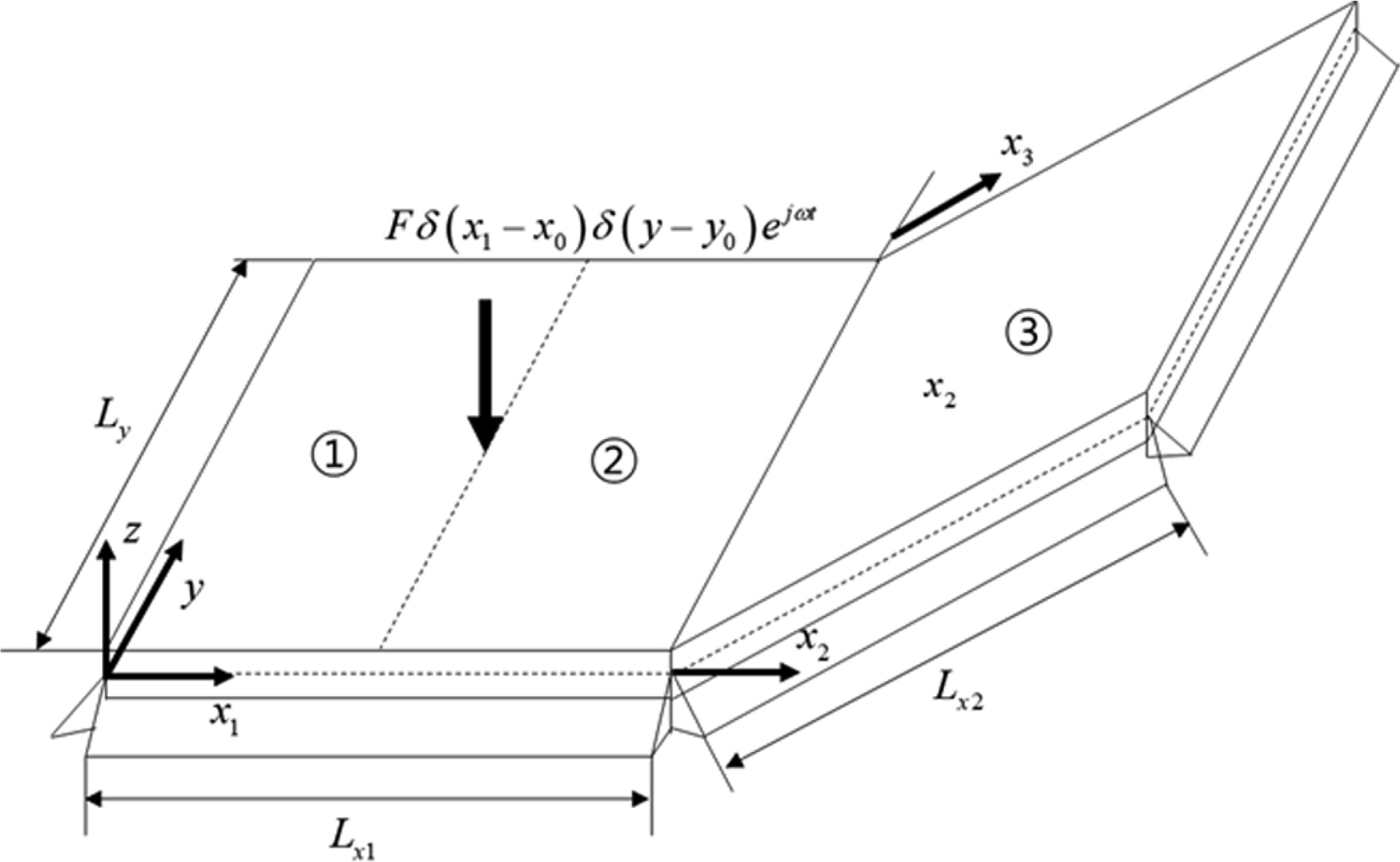
where C_m_,_i_,_n is the complex coefficient of the n^th-order mode, and H→_m_,_i_,_n and λ_m_,_i_,_n represent the n^th eigenvector and eigenvalue of matrices [N_m_,_i(ω)], respectively. The number of unknowns for each plate boundary of the plate structure in Fig. 1 is 4 flexural waves and 4 in-plane waves, requiring a total of 24 boundary conditions. The boundary conditions at x₁ = 0 are expressed as follows.

(20)

u1(0,y)=0

(21)

∂v1(0,y)∂x1=0

(22)

w1(0,y)=0

(23)

∂2w1(0,y)∂x12=0

The boundary conditions at the excitation-point locations of x₁ = x₀ and x₂ =− L_x₁ +x₀ are expressed as follows.

(24)

u1(x0,y)=u2(x0−Lx1,y)

(25)

v1(x0,y)=v2(x0−Lx1,y)

(26)

w1(x0,y)=w2(x0−Lx1,y)

(27)

∂w1(0,y)∂x1=∂w2(x0−Lx1,y)∂x1

(28)

Nxx,1(x0,y)=Nxx,2(x0−Lx1,y)

(29)

Nxy,1(x0,y)=Nxy,2(x0−Lx1,y)

(30)

Vxz,1(x0,y)+Fδ(y−y0)=Vxz,2(x0−Lx1,y)

(31)

Mxx,1(x0,y)=Mxx,2(x0−Lx1,y)

Here,

The boundary conditions at x₂= x₃= 0, where the two plates are coupled at an arbitrary angle, are expressed as follows.

(32)

u2(0,y)=−w3(0,y)sinθ+u3(0,y)cosθ

(33)

v2(0,y)=v3(0,y)

(34)

w2(0,y)=w3(0,y)cosθ+u3(0,y)sinθ

(35)

Nxx,2(0,y)=−Vxz,3(0,y)sinθ+Nxx,3(0,y)cosθ

(36)

Nxy,2(0,y)=Nxy,3(0,y)

(37)

Vxx,2(0,y)=Vxz,3(0,y)cosθ+Nxx,3(0,y)sinθ

(38)

∂w2(0,y)∂x2=∂w3(0,y)∂x3

(39)

M2(0,y)=M3(0,y)

Lastly, the four boundary conditions at x₃ = L_x₂ are expressed as follows (similar to the boundary conditions at x₁ = 0).

(40)

u3(Lx2,y)=0

(41)

∂v3(Lx2,y)∂x3=0

(42)

w3(Lx2,y)=0

(43)

∂2w3(Lx2,y)∂x32=0

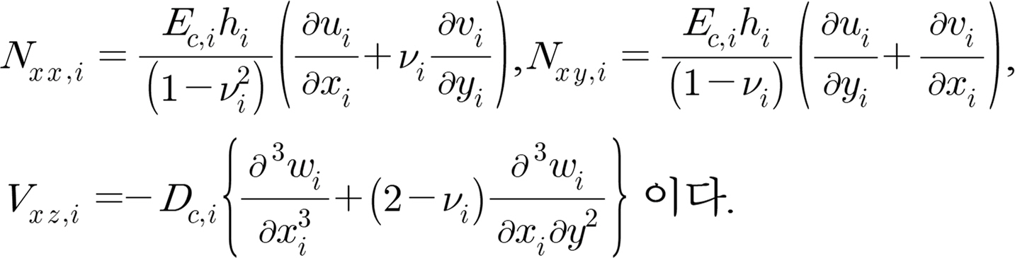
If the displacement solution is obtained using the foregoing boundary conditions, the energy density and vibration intensity of the flexural wave and the in-plane wave of the plate can be obtained using the following equations:

(44)

〈ef〉i=Di4{|∂2wi∂xi2|2+|∂2wi∂y2|2+2νi∂2wi∂xi2(∂2wi∂y2)* +2(1−νi)∂2wi∂xi∂y(∂2wi∂xi∂y)*}+ρihi4|∂wi∂t|2

(45)

〈qfx〉i=12Re{−Qxz,i(∂wi∂t)2+Mx,i(∂2wi∂xi∂t)*+Mxy,i(∂2wi∂yi∂t)*}

(46)

〈qfy〉i=12Re{−Qyz,i(∂wi∂t)2+My,i(∂2wi∂yi∂t)*+Myx,i(∂2wi∂xi∂t)*}

Here,

(47)

Mx,i=-Dc,i{∂2wi∂xi2+νi∂2wi∂yi2},My,i=-Dc,i{∂2wi∂yi2+νi∂2wi∂xi2},Mxy,i=Myx,i=-Dc,i(1-νi)∂2wi∂xi∂y,Qxz,i=-Dc,i{∂3wi∂xi3+νi∂3wi∂xiy2},Qyz,i=-Dc,i{∂3wi∂yi3+νi∂3wi∂xi2∂y}〈eI〉i=14Re[Gc,ihi|∂ui∂y+∂vi∂xi|2+Kc,i(∂ui∂xi+νi∂vi∂y)(∂ui∂xi)* +Kc,i(∂vi∂y+νi∂ui∂xi)(∂vi∂y)*+ρihi(|∂ui∂t|2+|∂vi∂t|2)]

(48)

〈qIx〉i=12Re[Gc,ihi(∂ui∂y+∂vi∂xi)(∂vi∂t)*+Kc,i(∂ui∂xi+νi∂vi∂y)(∂ui∂t)*]

(49)

〈qIy〉i=−12Re[Gc,ihi(∂ui∂y+∂vi∂xi)(∂vi∂t)*+Kc,i(∂ui∂y+νi∂vi∂xi)(∂ui∂t)*]

where G_c_,_i = E_c_,_i/{2(1+ν_i)} and Kc,i=Ec,ihi/(1−νi2)

4.2 Energy Flow Solution of Coupled-plate Structures

The energy flow solution of the coupled plate can be obtained as in previous studies (Park et al., 2001). The Levy series solution that satisfies the y-direction boundary condition of the energy governing equation in Eqs. (3), (4), and (6) was expressed, and the energy flow solution was calculated using the boundary condition of the wave solution in the x_i direction.

(55)

〈en〉i(xi,y)=∑m=0∞Em,n,i(xi)cos(kmy) (n=f,l,s)

Here, the wave solution of the energy density solution for each n-type wave is given by Eq. (45).

(56)

Em,n,i(xi)=Am,n,i+e−αm,n,ixi+Am,n,i−e−αm,n,ixi

Here, Am,n,i+ represents the m^th-order mode coefficient of the wave solution traveling in the n-type ± direction in the i-plate region, and Am,n,i+.

4.3 Energy Density Comparison of Coupled-plate Structures

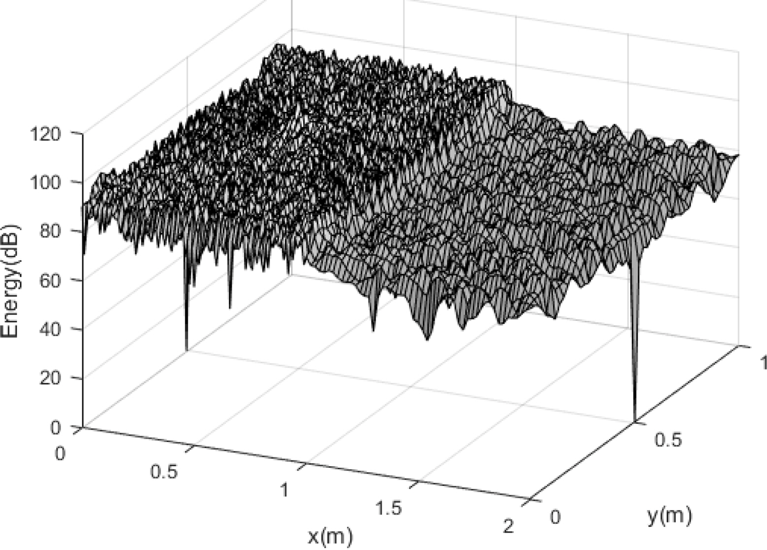
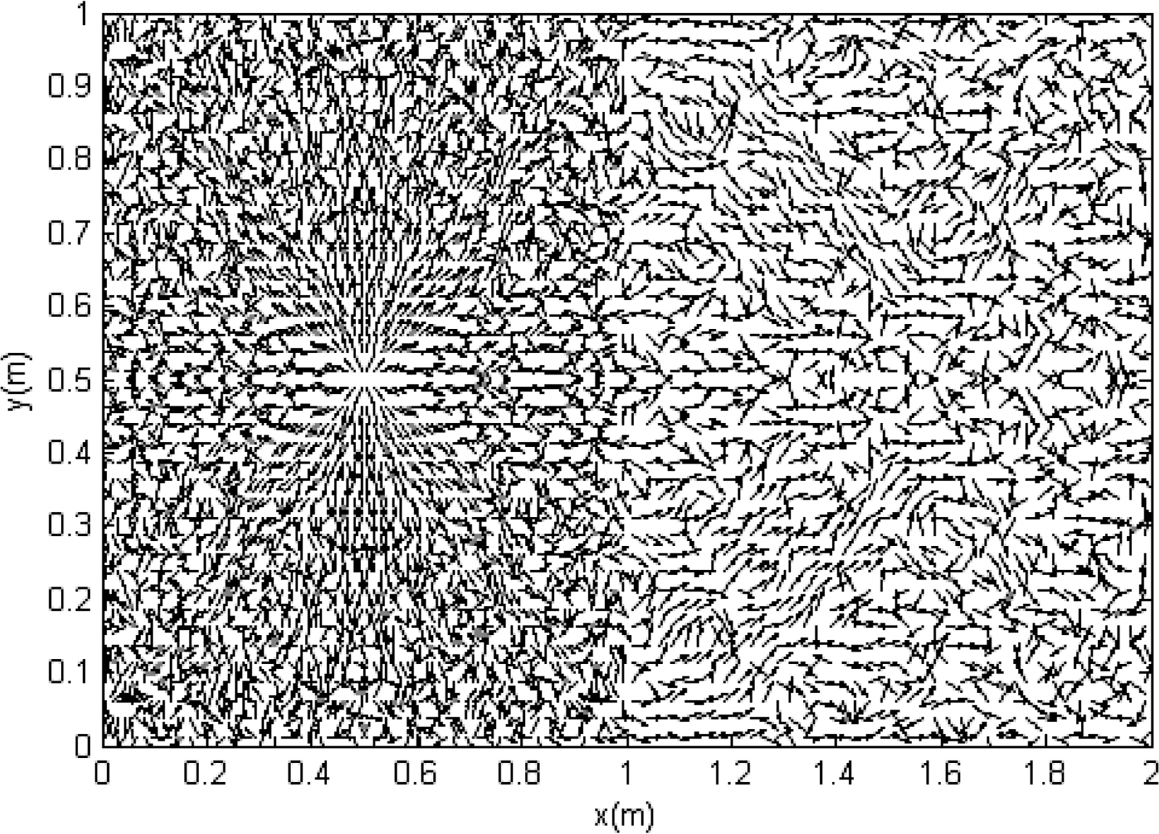
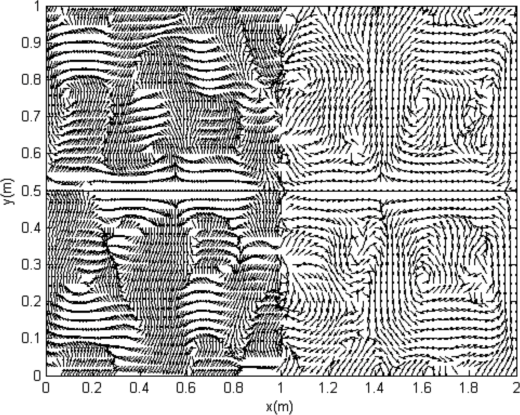
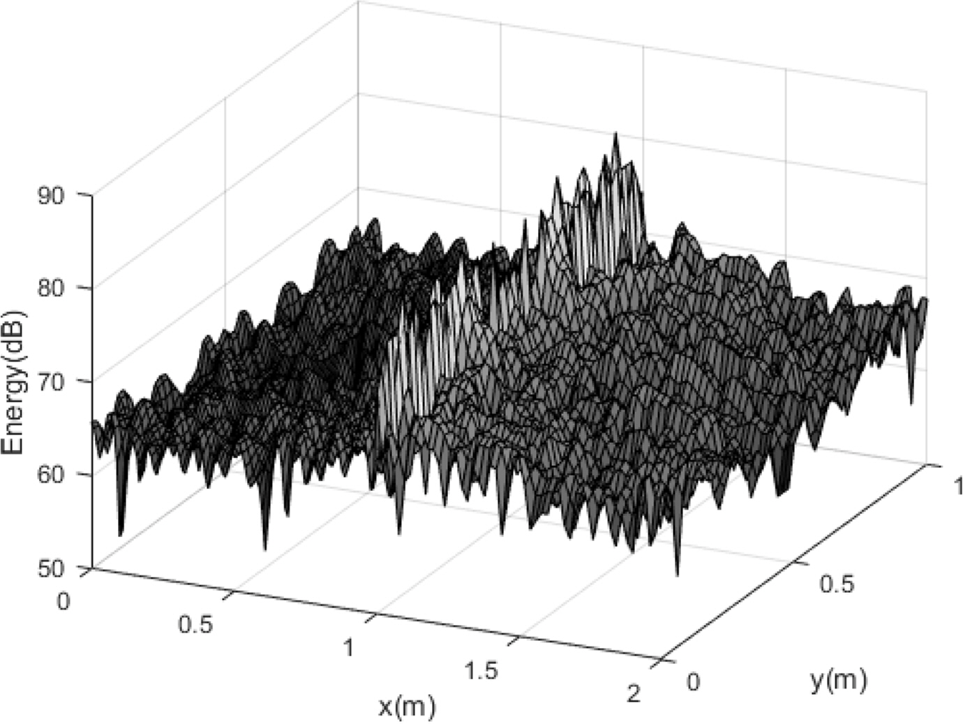
It was assumed that the size of the plate structure in Fig. 1 was L_x₁ = L_x₂ = L_y =1 m and that the coupled angle of the plate was 30°. The material of the plate was aluminum (E = 7.1 ×10¹⁰ N/m² and ρ = 2700 kg/m³), and the structural damping loss factor of the plate was set as η = 0.01 to express the spatial damping to a certain degree. All the plate thicknesses were h = 0.001 m. The vertical excitation force was applied to the center of the first plate position (L_x₁, Ly) = (0.5 m, 0.5 m), and the size was 10 N. The number of modes for obtaining an approximate solution was set as 200 to improve the accuracy of the analysis. The analysis results for an exact solution at an excitation frequency of 10 kHz are shown in Figs. 2,–5. The energy density of the flexural wave was the highest at the excitation point because the plate was excited with a vertical load, and it tended to decrease as the distance from the excitation point increased. Additionally, the plate had the highest energy density at the boundary where the plates were coupled at an arbitrary angle, because the in-plane wave was generated at the position where the two plates were coupled at an arbitrary angle (in contrast to the flexural wave), and the energy density decreased owing to the increased structural damping toward the inside of each plate. The propagation tendency of the vibration energy can be observed in the excitation part of the vibrational intensity distribution, as shown in Figs. 4 and 5. The modal density of the plate vibration mode with respect to the frequency is presented in Table 1. Although the theoretical modal density of a flexural wave is constant with respect to the frequency, the in-plane wave tended to increase in proportion to the frequency.

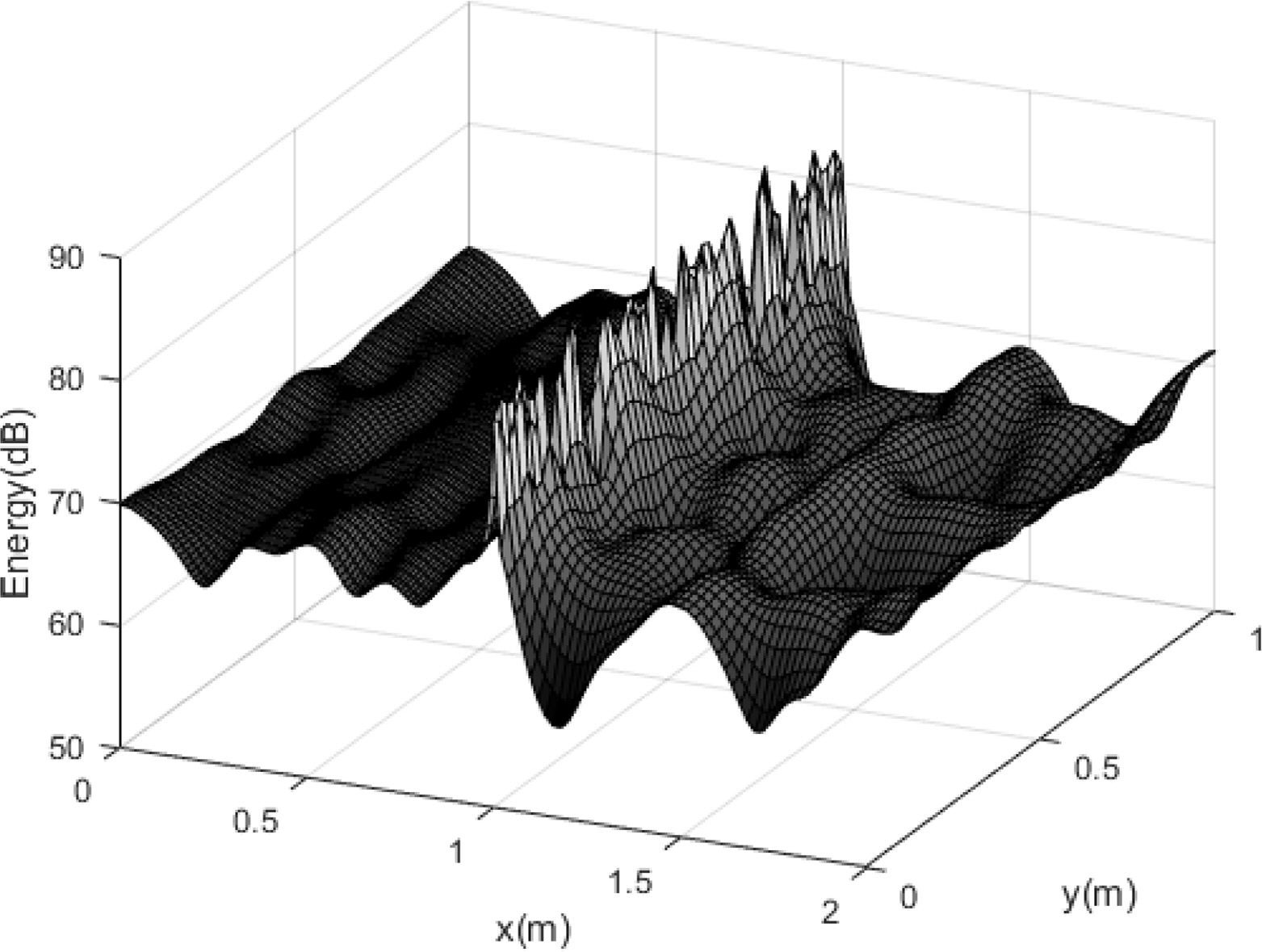
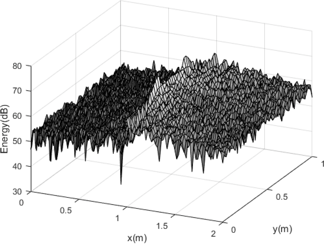
The effectiveness of the EFA, which is a statistical approach, increased in the high frequency range with a high modal density. The energy density distributions of in-plane waves for exact solutions at excitation frequencies of 30 and 100 kHz are shown in Figs. 6 and 7, respectively. The modal density increased with the frequency, increasing the mode superposition.

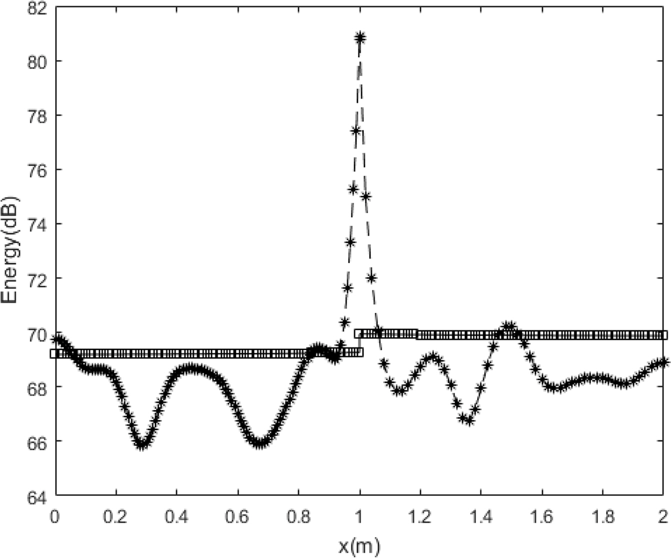
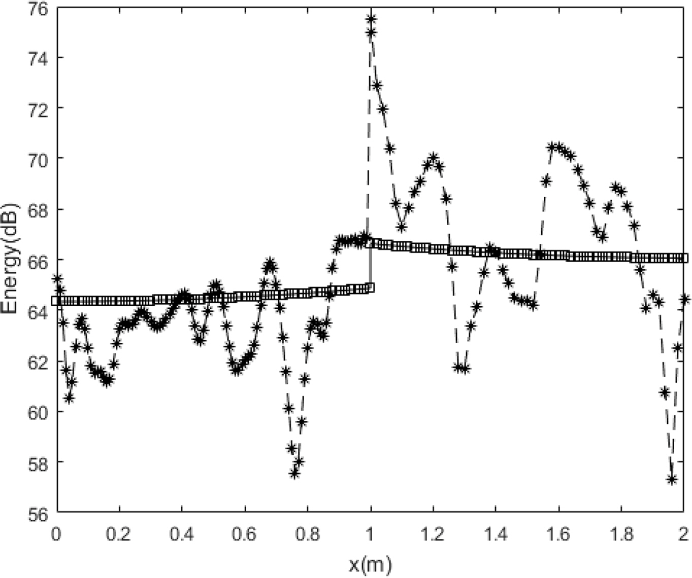
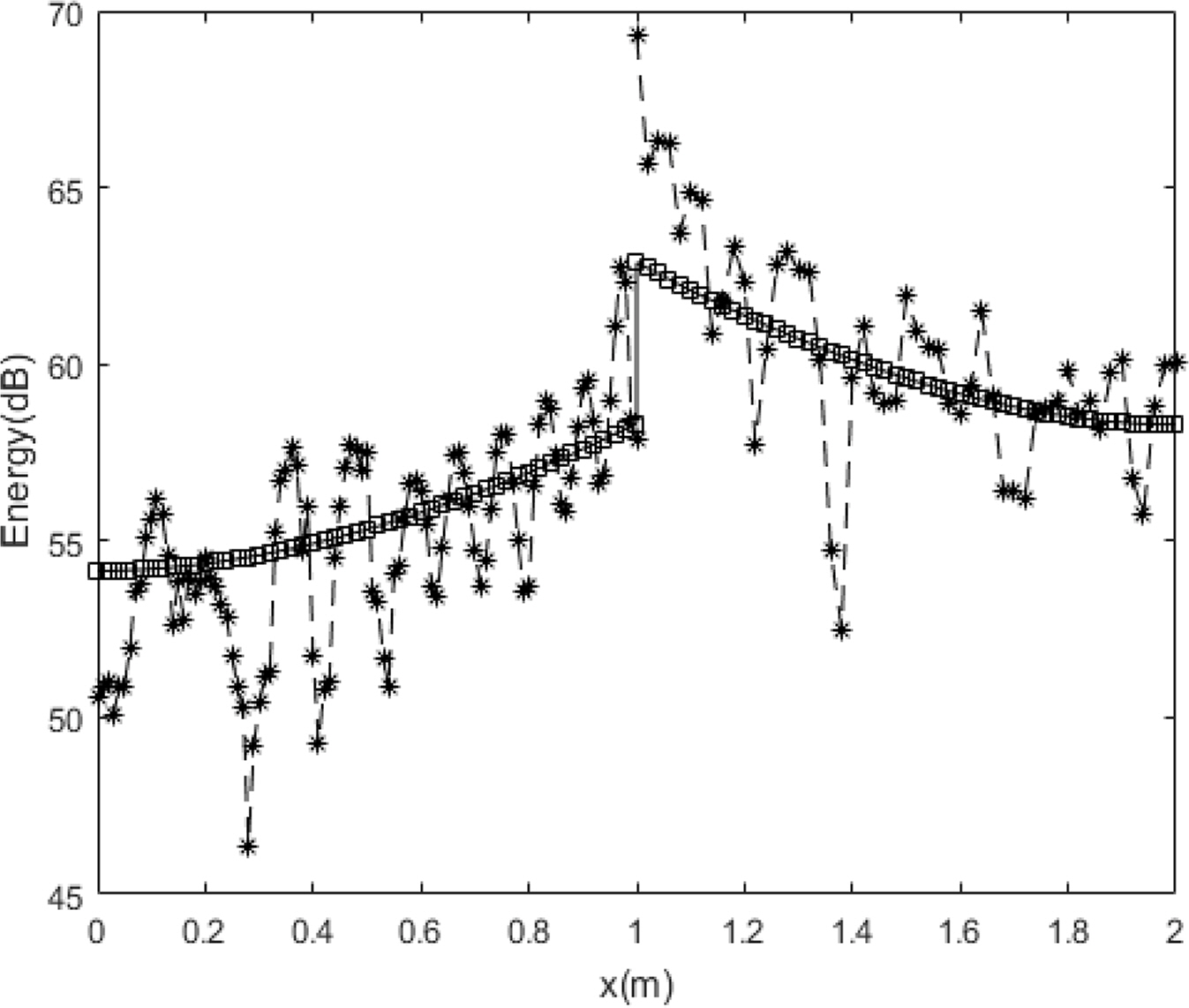
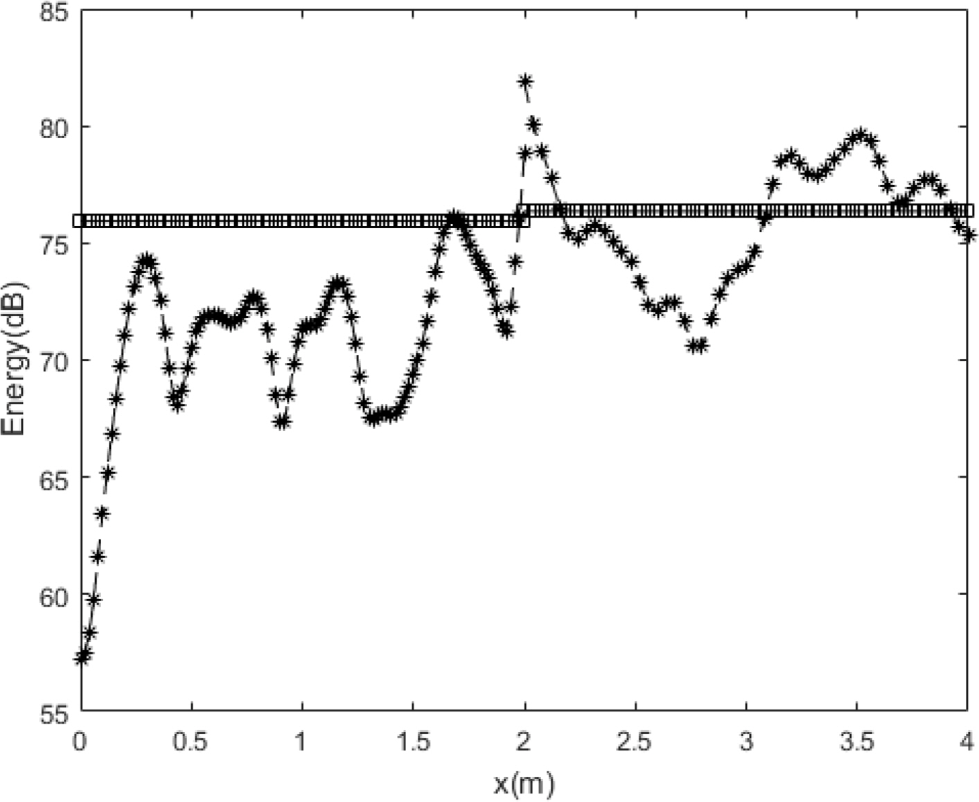
The comparison results for the energy density of the exact solution and the energy flow solution at different frequencies, with L_y = = 0.5 m, are shown in Figs. 8,–10.

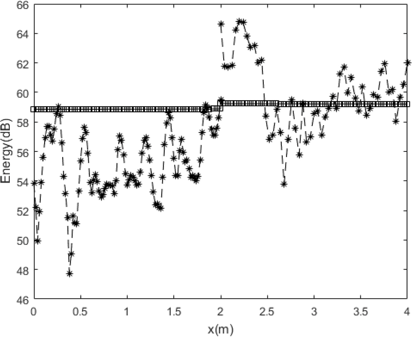
Compared with the flexural wave, the modal density was relatively low for the in-plane wave at the same frequency, as indicated by the foregoing analysis results. Therefore, although the exact solution and energy flow solution for the flexural wave in the previous studies had similar energy density distributions owing to mode superposition even in a relatively low frequency range, the spatial distributions of the energy density of the exact solution and the energy flow solution became similar at a significantly high frequency. However, the in-plane energy flow solution successfully showed the average distribution of the exact solution even in a relatively low frequency range, indicating that the EFA is extremely effective for predicting the overall vibration energy level in the middle–high frequency broadband. The size of the plate was doubled (L_x₁ = L_x₂ = L_y = 2 m) to examine the effects on the plate size, plate coupled angle, and structural damping loss factor, as shown in Figs. 11,–13, which present comparisons of the energy density between the exact solution and the EFA solution of the model with a plate coupled angle of 45° and a structural damping loss factor η = 0.001 for the plate material. Overall, the results were similar to those for the first example, even when the plate size, coupled angle, and structural damping loss factor were different.

5. Conclusion

In this study, the EFA, which is attracting attention as an effective vibration noise prediction method in the middle–high frequency ranges, was used to examine in-plane motions in coupled-plate structures. In previous studies, are view of the energetic characteristics depending on the frequency was performed by comparing the energy flow solution and the exact solution for the out-of-plane motion of the plate. However, a study on the reliability of the energy flow solution for in-plane motion was required, because no comparative review of in-plane motion had been conducted. In the present study, an EFA was performed to predict the average energy density level of the exact solution successfully for both out-of-plane and in-plane motions even in relatively low frequency ranges with a high out-of-plane modal density and low in-plane modal density. The EFA method is considered to be extremely effective for vibration analysis in the middle–high frequency ranges for engineers who are interested in the spatial distribution of the overall vibration energy level inside the structure rather than the spatial mode characteristics. In the future, the in-plane wave in the coupled model of the Mindlin plate, which has improved reliability in the high frequency range, must be verified.

Frequency (Hz)	Modal density (modes/Hz)

	Flexural	Longitudinal	Shear
10,000	0.3188	0.0064	0.0021
30,000	0.3188	0.0192	0.0064
100,000	0.3188	0.0636	0.0213