Study on PIV-Based Pressure Estimation Method of Wave Loading under a Fixed Deck

Article information

J. Ocean Eng. Technol. 2020;34(6):419-427

Publication date (electronic) : 2020 November 24

doi : https://doi.org/10.26748/KSOE.2020.059

Gang Nam Lee ¹

, Tien Trung Duong ²

, Kwang Hyo Jung ³^,

, Sung Bu Suh ⁴

, Jae Yong Lee ⁴

¹Post-doctoral Researcher, Department of Naval Architecture and Ocean Engineering, Pusan National University, Busan, Korea

²Graduate Student, Department of Naval Architecture and Ocean Engineering, Pusan National University, Busan, Korea

³Professor, Department of Naval Architecture and Ocean Engineering, Pusan National University, Busan, Korea

⁴Professor, Department of Naval Architecture and Ocean Engineering, Dong-Eui University, Busan, Korea

Corresponding author Kwang Hyo Jung: +82-51-510-2343, kjung@pusan.ac.kr

Received 2020 October 13; Revised 2020 October 25; Accepted 2020 October 27.

Abstract

In this study, a particle image velocimetry (PIV)-based pressure estimation method was investigated, with application to the wave-in-deck loading phenomenon. An experimental study was performed in a two-dimensional wave tank using a fixed deck structure under a focused wave, obtaining local pressures by pressure sensors, global loads by load cells, and instantaneous velocity fields using the PIV measurement technique. The PIV-based pressure estimation method was applied using the Euler equation as the governing equation, and the proper time step for the wave impact pressure was studied using the normalized root-mean-square deviation. The pressure estimation method showed good agreement for the local impact pressure in comparison with the measured pressure by the pressure sensors. However, some differences were observed in the peak pressure due to the limitations of the Euler equation and the sampling rate of the measurement system. Using the estimation method, the pressure fields during wave-in-deck loading were determined in the study, with an analysis of the mechanism of impact and negative pressure occurrence.

Keywords: PIV-based pressure estimation; Wave loading under deck; Euler equation; Focused wave; Pressure field

1. Introduction

Ships and offshore structures operating in harsh marine environments are easily exposed to wave impact loads such as green water and slamming due to high waves, and wave-in-deck loads of offshore structures. This can cause great damage to ships and offshore structures, or even cause capsizing (Faulkner, 2001; Ersdal and Kvitrud, 2000; Faltinsen, 2005; Kaiser et al., 2009). For the structural safety design of ships and offshore structures that can overcome the impact load caused by waves, the structural design criteria must first be established with an accurate estimation on the external force along with a quantitative understanding of the flow characteristics of the wave impact load. To this end, various experimental or numerical studies are being conducted to measure the pressure applied on the occurrence of wave impact loads and to quantitatively analyze the flow characteristics that cause them. The following representative studies have been conducted, and many other studies are currently being conducted: a study on the flow characteristics of the green water phenomenon that occurs in a simplified shape, and the measurement of the impact load by measuring the pressure applied on the deck and upper structure when a green water phenomenon occurs (Buchner and Voogt, 2000; Lim et al., 2012; Lee et al., 2020); an impact mechanism analysis using pressure measurement of the slamming phenomenon occurring at the leading edge, and a wedge-shaped model (Faltinsen et al., 2004; Shams et al., 2017; Oh and Jo, 2015; Xie et al., 2018); and an experimental pressure measurement and flow characteristics study on the wave-in-deck load (Abdussamie et al., 2014; Duong et al., 2019). Most of these studies experimentally measured and analyzed the pressure applied on the surface of the structure by using pressure sensors, and qualitative analysis was mainly performed on the flow characteristics that cause impact loads. However, it may be challenging to apply the Froude similarity when the impact pressure is measured using a pressure sensor (Rouse, 1959), which is widely used in experimental studies due to the nonlinearity and uncertainty of the phenomenon itself (Ariyarathne et al., 2012). In addition, the pressure sensors can only measure pressure locally, which can create flow disturbance due to direct contact between the fluid and the sensor. In order to solve these problems, a method of estimating the impact pressure using the surrounding flow velocity has been recently proposed (van Oudheusden, 2013). Thus far, the penetration method using conduction and resistance devices has mainly been used as an experimental method for measuring the flow velocity around ships and offshore structures, and a method using optical fibers has also been used (Chanson, 1997). However, these contact-type flow rate measurement methods generate disturbance of the surrounding flow due to direct contact with the fluid. Moreover, many non-contact flow rate measurement methods, which are used to measure the flow velocity through external optical image measurement, have been developed in order to overcome this shortcoming. Particle image velocimetry (PIV) is used to study the dynamics of various fluid properties, such as flow velocity and compressible fluids. PIV can be used to measure the position of particles in a fluid through optical image measurement without disturbing the flow, and to measure the velocity over the entire flow in the field of view at the same time. It is also used for high-precision verification of computational fluid dynamics (CFD) simulation, since it can provide the characteristics of the velocity field (Nila et al., 2013; Lee et al., 2016; Kim et al., 2019; Kim et al., 2020). This PIV-based velocity field measurement method can apply the Froude similarity to velocity, and can estimate the pressure field rather than the local pressure at the same time; thus, it is expanding its application range as an experimental pressure estimation method.

The pressure estimation method using the instantaneous velocity field measured through PIV was first applied in the field of aerodynamics. Van Oudheusden (2013) showed the applicability of the pressure and load estimation method through the flow field around the wing measured using PIV, and this pressure estimation method was applied to various shapes, including the wing (De Gregorio, 2006; Spedding and Hedenström, 2009). In the field of marine engineering, a study was conducted using the velocity field measured by PIV to calculate the internal pressure and acceleration of a fluid in waves (Jakobsen et al., 1997). Panciroli and Prfiri (2013) estimated the pressure during free fall of a wedge-shaped structure using the velocity field measured through PIV, and compared and verified the results with potential theory. Kim et al. (2020) investigated the damping mechanism in the roll motion of a rectangular-shaped structure in waves using the surrounding velocity field measured through PIV, and compared the estimated pressure with the CFD analysis results. These studies showed the accuracy and applicability of the pressure field estimation method using the velocity field measured using PIV.

In this study, the wave-in-deck load phenomenon was experimentally implemented, and a study was conducted on the application of the pressure estimation method using the instantaneous velocity field of the surrounding flow measured through PIV. A method of estimating pressure was proposed using the instantaneous velocity field of fluids based on the Euler equation, and measuring the local pressure for the wave impact load caused by the interference of the wave generated by the method of overlapping the regular wave with the deck structure fixed in the two-dimensional wave tank. The pressure estimation characteristics were compared depending on the time interval between the velocity fields for the instantaneous acceleration calculation, and a time interval setting method for accurate impact pressure estimation was proposed. In addition, a hydrodynamic analysis study was conducted on the mechanism of pressure generation of wave-in-deck loads by estimating the significant pressure field around the structure when an impact load occurs.

2. Theoretical Background

In order to estimate the pressure around the structure by using the instantaneous velocity field measured through PIV, the two- dimensional inviscid Euler equation is used as the governing equation in this study. The pressure gradient of the fluid in the PIV field of view can be estimated through the Euler equation-based Eqs. (1)–(2).

(1) ∂p∂x(x,z)=−ρDuDt=−ρ(∂u∂t+u∂u∂x+ω∂u∂z)

(2) ∂p∂x(x,z)=−ρDωDt=−ρg=−ρ(∂ω∂t+u∂ω∂x+ω∂ω∂z)−ρg

where p denotes pressure, ρ denotes fluid density, t denotes time, x and z denote the Cartesian coordinate systems in the horizontal and vertical directions, respectively, and u and w denote the instantaneous velocities for x and z, respectively. The spatial and temporal acceleration terms of the fluid at time t in Eqs. (1) and (2) were calculated by applying the central difference method (Eqs. (3), (4)) for the continuous velocity field measured through PIV, as shown in Fig. 1.

(3) ∂u∂x(x,z,t)=u(x+h,z,t)−u(x−h,z,t)2h

(4) ∂u∂t(x,z,t)=u(x,z,t+nδt)−u(x,z,t−nδt)2nδt

where δt denotes the time interval between images measured through PIV, h denotes the space interval between each vector, and n denotes the number of images between continuous velocity fields used in the acceleration calculation.

Fig. 1

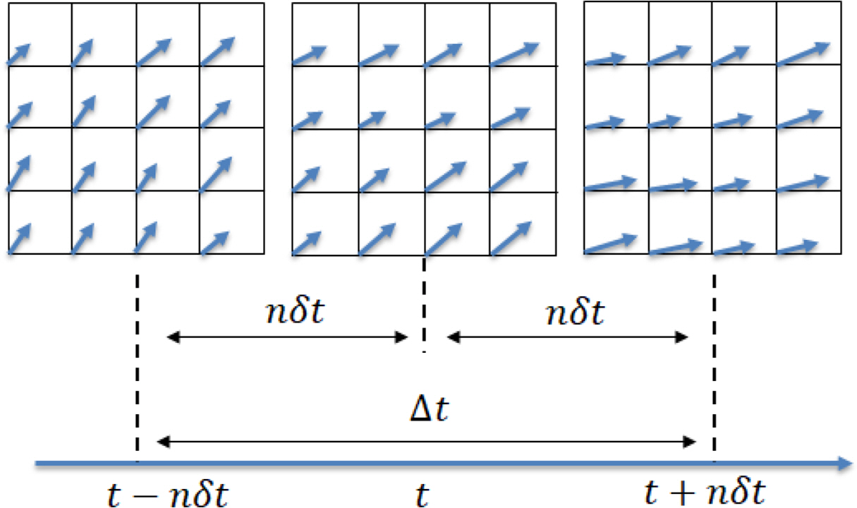
Time step between each velocity field for calculation of acceleration

The forward difference (Eq. (5)) and the backward difference (Eq. (6)) were used according to the location to calculate the spatial difference at the edge of the PIV field of view.

(5) ∂u∂x(x,z,t)=u(x+h,z,t)−u(z,x,t)h

(6) ∂u∂x(x,z,t)=u(x,z,t)−u(x−h,z,t)h

The pressure field of the fluid in the field of view was measured by applying spatial integration to the pressure gradient in the fluid field measured through the above process. The schematic spatial integration process is shown in Fig. 2. First, the pressure at the free surface is assumed to be atmospheric pressure, and the measured pressure gradient along the line L1 perpendicular to the x-axis direction is integrated for an arbitrary point A on the free surface. Then, the pressure for an arbitrary point B on the L1 line is measured through integration in the x direction and −x direction along L2 perpendicular to L1. Based on the measured pressures on L1 and L2, the space marching integral (Eq. (7)) (Baur and Köngeter, 1999) is used to measure the pressure of the rest of the field, as shown in Fig. 3. Next, the pressure field for a location other than point A on the free surface was measured in the same way, and the average value of each location of the pressure field measured in each measurement process was used as the final pressure field.

(7) p(s)=p(sref)+∫srefs∇p⋅ds

where S_ref denotes a reference position, and s denotes a spatial position to be calculated.

Fig. 2

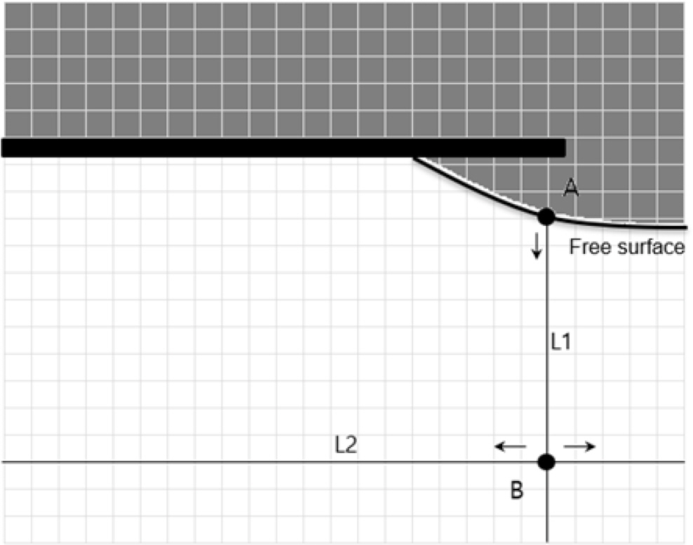
Pressure integration scheme in the study

Fig. 3

Spatial forward integration method

3. Wave-in-Deck Load Experiment Method

3.1 Experimental Conditions

In order to examine the accuracy of the PIV-based impact pressure estimation method, the results were compared and verified by applying it to a model experiment (Duong et al., 2019) for wave-in-deck loads. The model experiment was conducted in a two-dimensional wave tank (32 m long, 0.6 m wide, 1 m deep) equipped with a piston-type wave maker and an inclined wave absorber, as shown in Fig. 4. The dimension of the deck structure was determined by referring to a jacket-type structure operating in the Gulf of Suez area with a similar ratio of 1:56 (Table 1). In addition, the breadth of the structure was set to 0.60 m, equal to the breadth of the tank, in order to exclude the three-dimensional effect of the impact load phenomenon.

Fig. 4

Schematics of experimental setup

Table 1

Principal dimensions of prototype and model

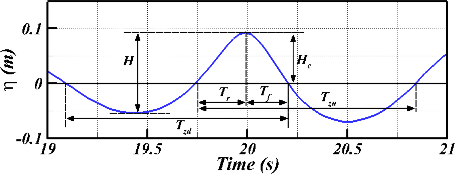
In this experiment, a focused wave made with two regular waves with having different periods and wave heights was used to implement the deck impact load in extreme environments and to exclude the effects of previous waves. The focused wave has a relatively strong nonlinearity compared to the regular waves, and the main variables for the wave height and period of each regular wave used for the focused wave and the wave nonlinearity (Myrhaug and Kjeldsen, 1986) are listed in Table 2. In this experiment, the velocity field and pressure were measured when the wave-in-deck load occurred due to the focused wave. The time series of the waves used is shown in Fig. 5, where H_c denotes the crest height, H_t denotes the trough height, H denotes the wave height, T_r and T_f denote the time taken for the wave to reach the crest from the average surface, and to reach the average surface from the crest, respectively, and T_zu and T_zd denote the zero up-crossing and zero down-crossing periods, respectively. Each variable is schematically shown in Fig. 5.

Table 2

Specifications of component and focused waves

Fig. 5

Time history of focused wave

The deck structure used in the experiment was fixed at a distance of 15 m from the wave maker, all experiments were conducted at a depth of 0.60 m, and measurements were performed immediately before the reflected wave from the wave absorber returned to the experiment site. Details on the experimental conditions and the implementation of overlapping waves are shown in Duong et al. (2019) and Duong (2019).

3.2 Pressure Measurement Method

Five pressure sensors were used to measure the wave impact load applied vertically on the lower deck (Fig. 6). A piezo-resistive type pressure gauge (Kistler 4043A2) that can measure both static and dynamic pressure at the same time was used as the pressure sensor, which was installed at five points in the center of the deck, spaced at equal intervals. The sampling rate of the pressure sensor was set to 5 kHz through a pre-convergence test for the impact load. Post-processing was performed using a finite impulse response (FIR) low-pass filter to remove noise from the measured pressure signal. The cutoff frequency and filter order of the FIR filter were 150 Hz and 91st order, respectively, using the method proposed by Lee et al. (2020).

Fig. 6

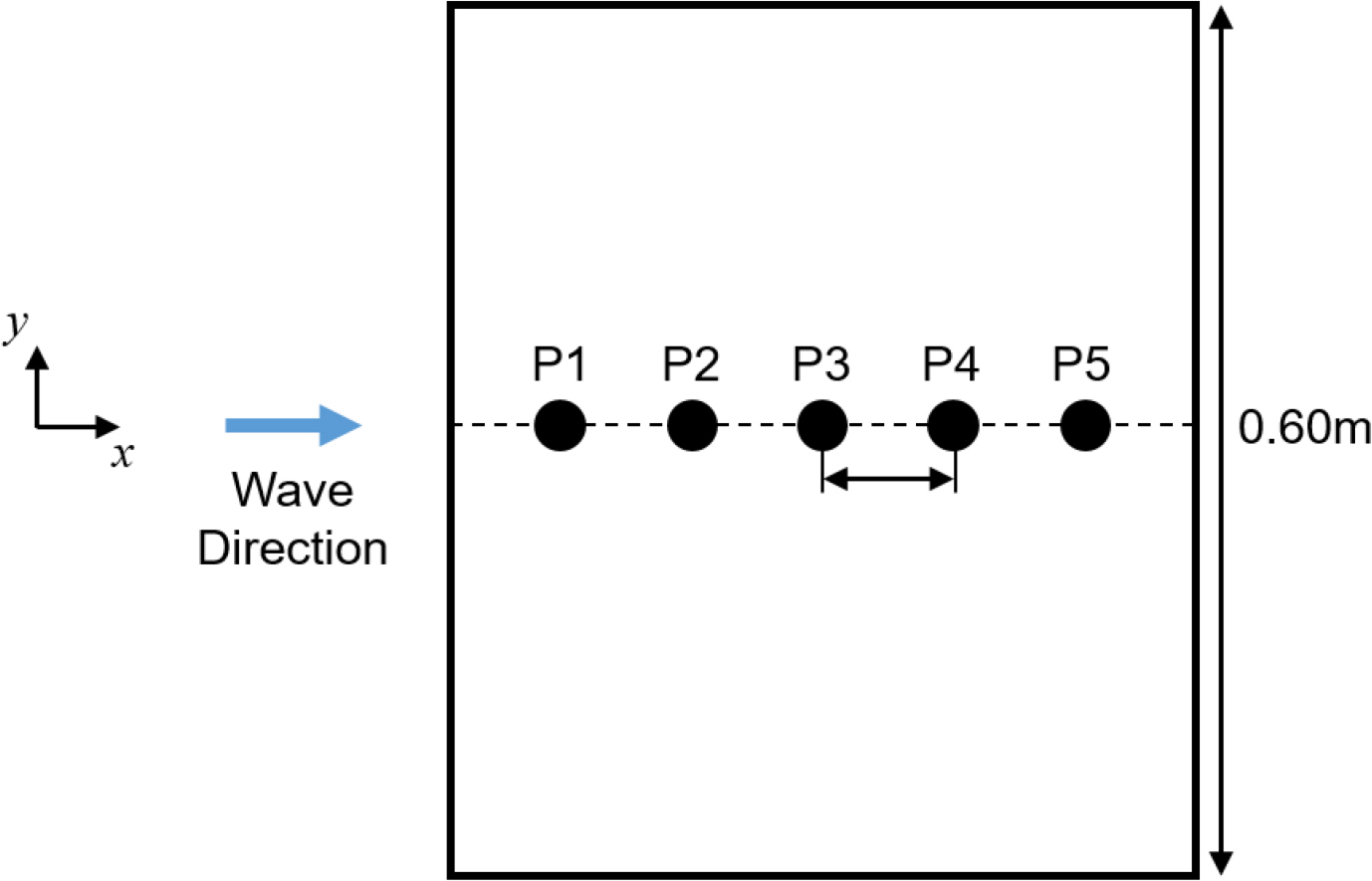
Location of pressure sensor installations

3.3 PIV Measurement Setup and Method

In this study, the PIV technique was applied for the measurement of the instantaneous velocity field around the structure when the wave-in-deck load was generated, as shown in Fig. 7. The particles used for PIV measurement had a neutral buoyancy of 57 µm in diameter and a specific gravity of 1.02. A continuous laser [maximum 8 W, wavelength (λ) 532 nm] was used as a light source for the reflection of the particles.

Fig. 7

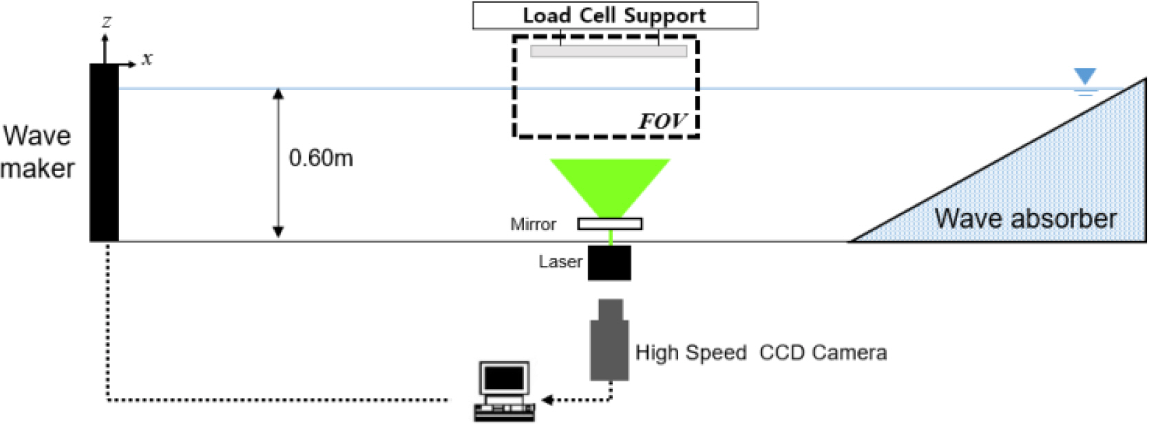
Experimental setup for PIV measurement

In terms of the PIV image, a high-speed charge-coupled device (CCD) camera (Redlake Y5) with a resolution of 2352 × 1728 pixels and a 105-mm optical lens (Nikkon, f# 2.8) were used to acquire 500 images per second (δt = 500 Hz) for a field of 0.44 × 0.32 m².

Adaptive cross-correlation (Theunissen et al., 2007, Eq. (8)) was used to increase the calculation accuracy by changing the size of the interrogation area to calculate the particle velocity for the measured image. The interrogation area was set to decrease from 256 × 256 pixels to 64 × 64 pixels, and the interval between the finally calculated velocity vectors was 5.95 mm by applying 50% overlap.

(8) C(Δx,Δy)=1MN∑i=0M−1∑j=0N−1f(m,n)g(m+Δx,n+Δy)

where C denotes the cross-correlation function, M and N denote the number of pixels in the x- and y-direction interrogation area, i and j denote the target image coordinates, and f and g denote the particle distribution of the continuous image.

The false vector in the velocity field was removed and post- processed through a median test (Westerweel, 1994), as expressed in Eq. (9) below.

(9) |U2D(median)−U2D(i,j)|<∊thresh

where U₂_D(n) denotes the surrounding vector, U2 D(i,j) denotes the test vector, and ∊_thresh denotes the limit value used for the test, which was set to 1.1 in this study.

The measurement error of the PIV measurement method is the sum of the bias error and the random error, which is expressed as a function of d_τ/d_pix by dividing the particle diameter (d_τ) in the image by the pixel interval (d_pix ) (Prasad et al., 1992). The term d_τ can be calculated as follows:

(10) dτ=(Mdp)2+ddiff2

where M denotes the ratio of the distance between the image and the lens, and the distance between the lens and the field of view; d_p denotes the actual diameter of the particle; and d_diff denotes the diameter of the particle observed in the image by laser diffraction (Hecht and Zajac, 1974), which is derived from Eq. (11).

(11) ddiff=2.44f(M+1)λ

The term d_τ/d_pix for the PIV measurement area used in this study was calculated to be approximately 0.09, and the corresponding measurement error was approximately 0.06 pixels (Raffel et al., 1998). In other words, it has a measurement error of approximately 2.55% of the local instantaneous maximum velocity (about 0.3 m/s) of the fluid measured through this PIV method.

4. Experimental Results

4.1 Comparison of Pressure Estimation Results According to Time Interval

The pressure estimation method using PIV proposed in this study may differ in accuracy and error depending on the time interval (Δt = 2nδt) between velocity fields used in the acceleration calculation. Therefore, the time interval selection for the pressure calculation should precede the pressure estimation for increased accuracy.

The pressure estimation results and the measurement results through the pressure sensor in P1 for the wave-in-deck load phenomenon according to the time interval change (2δt, 10δt, and 20δt) between the velocity fields for the acceleration calculation is shown in the time series in Fig. 8. The time (x-axis) was nondimensionalized to period of the zero down-crossing (T_zu) of the free surface of the wave, and the pressure (y-axis) was nondimensionalized to ρgH, as shown in Fig 8. The red dots are the pressure estimation results based on the PIV measurement velocity field, and the black solid line is the pressure measurement results measured by the pressure sensor in the model experiment. The pressure estimation results vary greatly depending on the change in δt. When δt is relatively small (Fig. 8(a), Δt = 2δt), a result close to the peak value of the shock pressure can be measured that rises momentarily when the wave hits the structure, but the estimated pressure results after the peak pressure fluctuate significantly. Conversely, when δt is relatively large (Fig. 8(c), Δt = 20δt), the estimated pressure generally matches well with the pressure measured through the pressure sensor, but shows a significant difference in the maximum value of the pressure. In other words, it was found that the accuracy of the velocity field-based pressure estimation method measured through PIV decreased as the time interval between velocity fields for the acceleration calculation became longer or shorter. This is believed to be due to the phenomenon that the accuracy error increases when the time interval between the velocity fields is short, and the truncation error increases as the time interval increases when calculating the acceleration using the velocity field (van Oudheusden, 2013).

Fig. 8

Comparison of estimated pressures and measured pressures at P1 with various time steps ((a) Δt = 2δt, (b) Δt = 10 δt, (c) Δt= 20δt)

The normalized root-mean-square deviation (NRMSD) of the measured pressure according to the change in time interval and the PIV-based estimated pressure were compared to determine the quantitative accuracy of the time interval between the velocity fields of the PIV-based pressure estimation method. NRMSD is calculated as follows:

(12) NRMSD=1n∑i=1n(pm,i−pc,i)2|pm,max−pm,min|

where p_m denotes the pressure measured through the pressure sensor, p_c denotes the estimated pressure using the PIV measurement results, and i denotes the discretized time.

The changes in NRMSD according to the number of images (n) between the velocity fields set for the acceleration calculation at each of the five pressure sensor installation positions are compared, as shown in Fig. 9. The NRMSD had the lowest value for n = 5 at all pressure sensor installation positions. This means that when the time interval between the velocity fields for acceleration calculation is 10δt, the result of the estimated pressure based on the PIV velocity field best matches the pressure measured by the pressure sensor. Based on this result, it was found that the time interval between the velocity fields of the PIV-based pressure estimation method for the wave-in-deck load showed the smallest difference from the pressure measurement results for Δt = 10δt. The NRMSD results proposed in this study are expected to show different results depending on the flow or pressure characteristics of each phenomenon to be estimated. In addition, it is determined that an appropriate time interval needs to be selected considering the characteristics of each phenomenon.

Fig. 9

NRMSD with different number of images between two velocity fields for calculation of acceleration (n)

4.2 Pressure Field Estimation Results for the Case of Wave Impact Load

Fig. 10 shows a comparison of the pressure obtained using the instantaneous velocity field based pressure estimation method measured through PIV and the measurement results through the pressure sensor for the wave-in-deck load when the time interval between the velocity fields is 10δt(n = 5). Overall, the instantaneous velocity field based pressure estimation method applied in this study produced results that are in good agreement with the measurement results through the sensors for the local pressure caused by the wave-in-deck load. The estimated results were close to the peak values of the impact pressure that increased for the short moment of the wave-in-deck load at each pressure measurement location. Afterward, the negative pressure generated due to the gradually decreased pressure as the wave moved away showed good agreement overall. However, the pressure was relatively low for the pressure measured by the sensors for the peak impact pressure that increased rapidly; in particular, the difference was greater for P1 and P2 located at the leading edge of the deck. This seems to be attributable to the truncation error that occurred due to the relatively large time interval between the instantaneous velocity fields measured by PIV compared to the rise time of the pressure when the impact phenomenon occurred. In addition, it is believed to have some differences, since the impact load estimation method used in this study did not consider the viscosity of the fluid based on the Euler equation.

Fig. 10

Time history of measured and estimated pressure

The pressure field under the deck estimated using the PIV measurement image and the velocity field of each occurrence of the wave-in-deck load are shown in Fig. 11. Each image of the contact at the leading edge (Fig. 11(a)), the moment the maximum pressure is measured at the pressure gauge measurement position (P1–P5) (Figs. 11(b)–11(f)), the emergence of the leading edge (Fig. 11(g)), and the moment the flow moves away from P1 according to the process of generating the wave-in-deck load are shown in Fig. 11. The x-axis is the length of the structure (L), the y-axis is the depth of water (D = 0.60 m), the velocity is L/T_zu, and the pressure is ρg H nondimensionalized, as shown in Fig. 11.

Fig. 11

Pressure and velocity fields under the deck at various wave phases

At the contact at the leading edge (Fig. 11(a)), the pressure due to the waves begins to be applied to the structure, and this pressure increases gradually as the waves cross under the deck and propagate to the trailing edge of the deck. At the moment when the local pressure at the position of each pressure sensor peaks (Figs. 11(b)–11(f)), it is observed that the pressure of the surrounding fluid increases significantly at the same time. It was also found that the flow velocity around the contact area accelerated in the horizontal direction. It is believed that the free surface was deformed by the structure, momentarily impacting the structure, and a jet phenomenon, in which fluid is accelerated, occurred at the same time. In addition, it is found that the fluid pressure is smaller at the emergence of a leading edge (Figs. 11(e)–11(f)) than the pressure at the moment the wave first impacts the leading edge of the structure (Figs. 11(b)–11(d)) as the wave energy is transmitted to the structure as an impact when the wave crosses along the lower deck. At the emergence of the leading edge (Fig. 11(g)), it is seen that a negative pressure lower than atmospheric pressure occurs from the leading edge of the structure above the free surface. This continues until the moment P1 is exposed to the atmosphere (Fig. 11(h)), and then the pressure at the bottom of the lead becomes equal to the atmospheric pressure as the wave moves away from the structure.

5. Conclusion

In this study, the pressure measured through pressure sensors, and the velocity field-based pressure estimation results were compared and analyzed. This was accomplished by applying a method for estimating fluid pressure using the instantaneous velocity field measured through PIV based on Euler’s equation to the wave impact load test under the deck conducted in a two-dimensional wave tank.

It was found that the pressure estimation results of the velocity field based pressure estimation method applied in this study were significantly different according to the time interval (Δt) between velocity fields for the acceleration calculation.When the time interval was short, the peak value of the instantaneously high impact pressure caused by the impact load was estimated well, but the overall pressure fluctuated due to an increase in the accuracy error. Moreover, the overall pressure was estimated well as the time interval increased, but the truncation error increased, resulting in a difference in the maximum value of the instantaneous impact pressure.

In order to set an appropriate time interval to improve the accuracy of the velocity field based pressure estimation method, this study utilized the NRMSD to examine the quantitative error of the pressure estimation method. As a result, it was found that the wave-in-deck load had the lowest error at 10. However, the NRMSD must vary according to the flow and pressure characteristics of each phenomenon to be estimated, and an appropriate time interval for each phenomenon must be estimated using the NRMSD.

In addition, it was found that the size of the maximum value of the impact pressure of the pressure estimation method based on the velocity field was slightly different compared to the pressure results measured by the pressure sensors. This seems to be attributable to the truncation error due to the relatively large time interval between the instantaneous velocity fields measured by PIV compared to the rise time of the impact pressure, which is believed to be the limitation of this method based on the Euler equation.

The pressure field around the structure during the wave-in-deck load was estimated and presented using the instantaneous velocity field. Through the pressure field, the hydrodynamic characteristics of the surrounding fluid were analyzed when an impact phenomenon caused by waves occurred, and the mechanism of occurrence of impact pressure and negative pressure was found through the relation with the velocity field.

The pressure field estimation method based on the instantaneous velocity field measured by using the PIV method can not only estimate the impact pressure without a pressure sensor, but it also has the advantage of being able to measure the pressure field without disturbing the flow in a wider range than conventional pressure sensors, which only measure local pressure. It is believed that this approach can be widely used not only for the fluid dynamic characteristics of complex fluid phenomena, such as impact phenomena, but also for the analysis of pressure generation mechanisms.

Acknowledgements

This work was supported by a 2-Year Research Grant of Pusan National University.

Notes

Conflict of interest

No potential conflict of interest relevant to this article was reported.

References

Abdussamie N, Thomas G, Amin W, Ojeda R. 2014. Wave-in-Deck Forces on Fixed Horizontal Decks of Offshore Platforms. In : Proceedings of the 33rd International Conference on Ocean, Offshore and Arctic Engineering. San Francisco, USA. p. 1–11. https://doi.org/10.1115/OMAE2014-23629 .

Ariyarathne K, Chang KA, Mercier R. 2012;Green Water Impact Pressure on a Three-dimensional Model Structure. Experiments in Fluids 53(6):1879–1894. https://doi.org/10.1007/s00348-012-1399-9 .

Baur T, Kongeter J. 1999. PIV with High Temporal Resolution for the Determination of Local Pressure Reductions from Coherent Turbulent Phenomena. In : Proceedings of 3rd Internatinal Workshop on Particle Image Velocimetry. Santa Barbara, USA. p. 101–106.

Buchner B, Voogt A. 2000. The Effect of Bow Flare Angle on FPSO Green Water Loading. In : Proceedings of ETCE/OMAE2000 Joint Conference, Energy for the New Millenium; 14–17 February 2000;

Chanson H. 1997. Air Bubble Entrainment in Free-surface Turbulent Shear Flows Academic Press Inc. https://doi.org/10.1016/B978-0-12-168110-4.X5000-0 .

De Gregorio F. 2006. Aerodynamic Performance Degradation Induced by Ice Accretion. PIV Technique Assessment in Icing wind Tunnel. In : Proceedings of 13th International Symposium Applications of Laser Techniques to Fluid Mechanics. Lisbon, Portugal.

Duong TT. 2019. Experimental Study of Wave Impact under Deck due to Focused Waves (Thesis for Master degree) Pusan National University; Busan, Korea:

Duong TT, Jung KH, Lee GN, Kim DS, Suh SB, Kim MS. 2019;Experimental Study on Wave Impact under Deck due to Regular Waves. Journal of Coastal Research 91(SI):81–85. https://doi.org/10.2112/SI91-017.1 .

Ersdal G, Kvitrud A. 2000. Green Water Incidents on Norwegian Production Ships. In : Proceedings of the 10th International Conference on Offshore and Polar Engineering (ISOPE 2000). Seattle, USA. 1p. 211–218.

Faulkner DJ. 2001. Survival Design of Cargo Hatch Structures. In : Proceedings of RINA Conference Design and Operation for Abnormal Conditions II. London, United Kingdom.

Faltinsen OM, Landrini M, Greco M. 2004;Slamming in Marine Application. Journal of Engineering Mathematics 48:187–217. https://doi.org/10.1023/B:engi.0000018188.68304.ae .

Faltinsen OM. 2005. Hydrodynamics of High-speed Marine Vehicles Cambridge University Press. New York:

Hecht E, Zajac A. 1974. Optics (Addison-Wesley Series in Physics) Addison-Wesley Pub. Co.

Jakobsen ML, Dewhirst TP, Greated CA. 1997;Particle Image Velocimetry for Predictions of Acceleration Fields and Forces within Fluid Flows. Measurement Science and Technology 8(12):1502–1516.

Kaiser MJ, Yu Y, Jablonowski CJ. 2009;Modeling Lost Production from Destroyed Platforms in the 2004–2005 Gulf of Mexico Hurricane Seasons. Energy 34(9):1156–1171. https://doi.org/10.1016/j.energy.2009.04.032 .

Kim MG, Jung KH, Park SB, Suh SB, Park IR, Kim J, Kim KS. 2019;Experimental Study on Viscous Effect in Roll and Heave Motions of a Rectangular Structure. Ocean Engineering 171:250–258. https://doi.org/10.1016/j.oceaneng.2018.11.004 .

Kim MG, Jung KH, Park SB, Lee GN, Duong TT, Suh SB, Park IR. 2020;Experimental and Numerical Estimation on Roll Damping and Pressure on a 2-D Rectangular Structure in Free Roll Decay Test. Ocean Engineering 196(15):106801. https://doi.org/10.1016/j.oceaneng.2019.106801 .

Lee GN, Jung KH, Chae YJ, Park IR, Malenica S, Chung YS. 2016;Experimental and Numerical Study of the Behaviour and Flow Kinematics of the Formation of Green Water on a Rectangular Structure. Brodogradnja : Teorija i praksa brodogradnje i pomorske tehnike 67(3):133–145. https://doi.org/10.21278/brod67308 .

Lee GN, Jung KH, Malenica S, Chung YS, Suh SB, Kim MS, Choi YH. 2020;Experimental Study on Flow Kinematics and Pressure Distribution of Green Water on a Rectangular Structure. Ocean Engineering 195:106649. https://doi.org/10.1016/j.oceaneng.2019.106649 .

Lim HJ, Park SH, Rhee SH. 2012;Experiments and Numerical Validation for FPSO Bow Water Shipping. Journal of the Society of Naval Architects of Korea 49(1):6–13. https://doi.org/10.3744/SNAK.2012.49.1.6 .

Myrhaug D, Kjeldsen SP. 1986;Steepness and Asymmetry of Extreme Waves and the Highest Waves in Deep Water. Ocean Engineering 13(6):549–568. https://doi.org/10.1016/0029-8018(86)90039-9 .

Nila A, Vanlanduit S, Vepa S, Van Paepegem W. 2013;A PIV-based Method for Estimating Lamming Loads during Water Entry of Rrigid Bodies. Measurement Science and Technology 23(4):045303.

Oh SJ, Jo DH. 2015;An Experimental Study on the Slamming Impact around Wedged type Structure in Accordance with the Weight and Height of the Change. Journal of Navigation and Port Research 39(1):77–82. https://doi.org/10.5394/KINPR.2015.39.1.77 .

Panciroli R, Porfiri M. 2013;Evaluation of the Pressure Field on a Rigid Body Entering a Quiescent Fluid Through Particle Image Velocimetry. Experiments in Fluids 54:1630. https://doi.org/10.1007/s00348-013-1630-3 .

Prasad AK, Adrian RJ, Landreth CC, Offutt PW. 1992;Effect of Resolution on the Speed and Accuracy of Particle Image Velocimetry Interrogations. Experiments in Fluids 13:105–116. https://doi.org/10.1007/BF00218156 .

Raffel M, Willert CE, Kompenhans J. 1998. Mathematical Background of Statistical PIV Evaluation Particle Image Velocimetry Experimental Fluid Mechanics Springer. Berlin, Heidelberg: https://doi.org/10.1007/978-3-662-03637-2_3 .

Rouse H. 1959. Advanced Mechanics of Fluids New York: John Wiley.

Shams A, Zhao S, Porfiri M. 2017;Hydroelastic Slamming of Flexible Wedges: Modeling and Experiments from Water Entry to Exit. Physics of Fluids 29(3):037107. https://doi.org/10.1063/1.4978631 .

Spedding GR, Hedenström A. 2009;PIV-based Investigations of Animal Flight. Experiments in Fluids 46:749–763. https://doi.org/10.1007/s00348-008-0597-y .

Theunissen R, Scarano F, Riethmuller ML. 2007;An Adaptive Sapling and Windowing Interrogation Method in PIV. Measurement Science and Technology 18(1):275–287.

Van Oudheusden BW. 2013;PIV-based Pressure Measurement. Measurement Science and Technology 24(3):032001.

Westerweel J. 1994;Efficient Detection of Spurious Vectors in Particle Image Velocimetry Data. Experiments in Fluids 16:236–247. https://doi.org/10.1007/BF00206543 .

Xie H, Ren H, Deng B, Tang H. 2018;Experimental Drop Test Investigation into Slamming Loads on a Truncated 3D Bow Flare Model. Ocean Engineering 169:567–585. https://doi.org/10.1016/j.oceaneng.2018.10.003 .

Article information Continued

This is an open access article distributed under the terms of the creative commons attribution non-commercial license (http://creativecommons.org/licenses/by-nc/4.0) which permits unrestricted non-commercial use, distribution, and reproduction in any medium, provided the original work is properly cited.

	Prototype	Model
Length (m)	22.00	0.40
Breadth (m)	18.00	0.60
Water depth (m)	33.50	0.60
Deck clearance (m)	4.56	0.06

Component 1		Component 2

Period (s)	Height (m)	Period (s)	Height (m)
1.04	0.108	1.25	0.109

Focused Wave

H_c(m)	H_t(m)	H(m)	T_r(s)	T_f(s)	T_zd(s)	T_zu(s)
0.093	0.054	0.047	0.25	0.22	1.11	1.10