


1. Introduction
Vessels located in a marine environment move in six degrees of freedom (6DOF). Among the 6DOF motions, the roll determines the boarding comfort, stability, and work environment of the passengers. Moreover, roll motions are associated with marine accidents such as ship overturn, which cause more material and human damage than ship engine failures. To prevent such marine accidents, there is a need for a process to identify the stability in waves in the ship design stage. As the stability of vessels is determined by the response amplitude operator (RAO) and wave energy spectrum of the floating body, it is critical to determine the RAOs of vessels. Existing methods to determine the RAO include experimental methods and computer analysis simulations. The determination of an RAO through experiments involves difficulties, owing to various constraints in the experimental model, equipment, and environment. To determine the RAO using computer simulations, the following three steps are required.
Step 1: A modeling process is conducted for the information of the vessel. This is a preliminary step for analysis and simulation, in which the shape information of the ship is generated.
Step 2: The vessel conditions are set. For example, the center of gravity and radius of gyration are input, considering the loading conditions and shape information of the vessel.
Step 3: The motion responses are analyzed in the frequency domain. Then, the analysis results (such as the RAO per external force direction) can be obtained.
However, the shape information of vessels is not easy to obtain, and some small and medium vessels do not have detailed information (e.g., drawings). Furthermore, computer simulation methods have inefficient aspects, as the above three steps must be repeated when the shape of the vessel changes. In addition, users have different skill levels for the commercial tools used in simulation, affecting the reliability of the results.
In view of the rising interest in artificial intelligence (AI)-related research in various fields, the shipbuilding and marine industry is also conducting research using AI techniques. Ham (2016) predicted lead times by considering the specifications and supply routes of fittings in shipyards using data mining techniques. Kim (2018) verified and discussed prediction models for production lead times by considering the properties of blocks and pipes among the data of shipyards. In terms of ship operations, Park et al. (2004) and Lee et al. (2005) evaluated stability to disturbances during the navigation of specific vessels using a 3D panel method and researched a system for evaluating an optimal sea route by setting the kinematic phenomena of the hull (such as excessive rolling phenomenon) as variables. Mahfouz (2004) defined parameters related to a nonlinear roll to predict a nonlinear roll time series for vessels, and measured the accuracy using a cross-validation function and applying a regression algorithm. Kang et al. (2012) used artificial neural network (ANN) techniques to predict, in real time, the responses of floating bodies to nonlinear waves. Kim et al. (2018) predicted the roll motions of 9600TEU container ships in operation using navigation variables. Kim (2019) developed a fuel consumption rate prediction model based on ship operation data and created and verified a decision support model for abnormal conditions of equipment on sailing ships. Kim et al. (2019) tested seakeeping performance by using the RAO at various incident angles. Jeon (2019) developed a meta-model by combining three machine learning models to predict the fuel consumption of vessels and validated the AI model.
Most studies combining the motions of vessels with AI techniques have investigated the optimal route, motion responses, and other topics regarding one specific vessel. However, this study aimed to predict the motion characteristics of specific vessels by learning the motion characteristics of barge-type ships with various specifications. First, information on barge-type ships registered with classification societies was collected. Then, the RAO data of each ship was generated using an in-house code, based on a 3D singularity distribution method. Thus, data sets of the specifications and RAOs were created for various barge-type ships. Using some of this data as training data, the RAOs of specific ships in the test data were predicted after a learning process. The ultimate goal of this study was to identify the roll RAOs of barge-type ships using AI techniques. The results of this study can provide a means for assessing the stability of various barge-type ships. Furthermore, the method developed in this study has the advantage of minimizing the modeling process for analyzing the RAO and the dependence on skill level for commercial tools.
2. Research Process
2.1 Machine Learning
Machine learning can be defined as a science of programming computers to learn from data. As shown in Fig. 1, machine learning can be classified based on the existence or absence of labeled data, into supervised learning, unsupervised learning, and reinforcement learning. Among them, supervised learning consists of classification and regression depending on predictions from results. Unsupervised learning is a method of deriving a result by a computer alone, i.e., without human intervention. One representative example of unsupervised learning is clustering. Reinforcement learning is a learning method that reinforces actions in the direction of the current action or in the opposite direction, through reward or penalty. Thus, this learning method selects an action or measure that maximizes the reward for selectable actions, by recognizing the current condition. The present study used a supervised learning method (which provides an answer) from among the machine learning methods, and a regression method to predict the values.
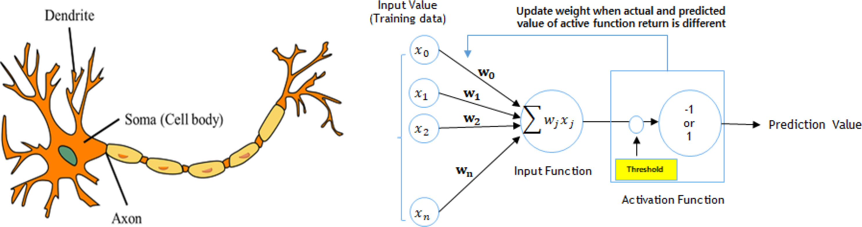
2.2 Perceptron
The human brain consists of combinations of neurons, and signals and information are communicated and learned through synapses interconnecting the neurons. A mathematical model of this process is called perceptron. Similar to the brainŌĆÖs learning principles, perceptrons also have the ability to solve problems by adjusting weights through learning. Fig. 2 shows conceptual diagrams of the human brain and perceptrons. The operation sequence of a perceptron is described below. However, single-layer perceptrons have difficulty in learning non-linear models, as there is only one activation function.
(1) Input of training data (x0, x1, x2 ŌĆ” xn);
(2) Multiplication of the weights (w0, w1, w2 ŌĆ” wn) and input value;
(3) Delivery of the sum of the multiplications to a net input function;
(4) Returning a ŌĆ£1ŌĆØ if the prediction data of the net input function is larger than the threshold of the activation function, or a ŌĆ£ŌłÆ1ŌĆØ if the former is smaller than the latter; and
(5) Updating the weight in the direction that minimizes the prediction and observation data.
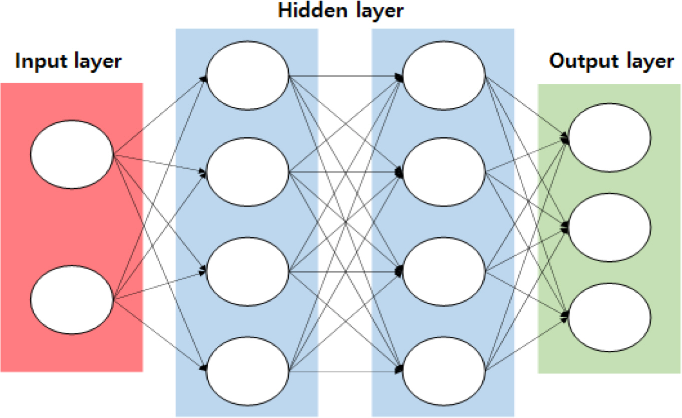
2.3 Multi-Layer Perceptron (MLP)
Fig. 3 shows a concept diagram of a multi-layer perceptron (MLP). An MLP consists of multiple hidden layers between the input and output layers to compensate for the above-mentioned disadvantages of the single-layer perceptron. The complexity of the neural network is determined by the number of hidden layers. An ANN with two or more hidden layers is generally called a deep neural network (DNN). The operation principle of an MLP is similar to that of a single-layer perceptron, and its sequence is as follows.
(1) Enter the training data (x0, x1, x2 ŌĆ” xn);
(2) Randomly set the weights of each layer (w0, w1, w2 ŌĆ” wn);
(3) Calculate the net input function value for each layer and the output value by the activation function;
(4) Update the weights until the difference between prediction and observation data by the activation function of the output layer becomes the tolerance; and
(5) Finish learning when the defined number of learning iterations for the training data is reached.
2.4 Data Collection
The length, breadth, and draft data of ships were collected from the specifications of barge-type ships registered with the Korea, Japan and Denmark-Germany register of shipping. In total, data were collected for 500 ships; ships with duplicate specifications were excluded from the data collection. In addition, eight input variables were generated for the learning model based on the collected ship data. The input variables were selected based on factors related to the roll motion, as shown in Table 1. The radius of gyration was set to 0.4 times the ship breadth, and the center of gravity was estimated under the assumption that the ship was on a free water surface.
2.5 Structure of Artificial Neural Network (ANN)
The learning model was created using the Python language, and the ANN was configured using the TensorFlow library. The hyperparameters used in this learning model are listed in Table 2. In addition, the numbers of hidden layers and hidden layer neurons were set as variables in this study. To prevent the overfitting of the ANN, the effects of the input variables were set identically through a normalization process of the input variables, and the range of normalization was set from 0 to 1. In addition, to prevent overfitting owing to the increased number of features during learning, the features of the learning model were reduced by applying the drop-out technique.
3. Learning Result and Discussion
3.1 Accuracy Assessment Indices
3.1.1 Random number change of the learning model
It was assumed that there would be a difference in the accuracy of the learning model depending on the training and test data, as data for a limited number of ships (500EA) was used. Thus, to consider various combinations of training and assessment data, the mean value of the accuracy was calculated for various training and assessment data, by changing the random number inside the learning model. In particular, the training and test data for the ANN were varied based on the seed number. Twenty random numbers from 0 to 19 were set, and the compositions of the assessment and test data were changed for each random number. Finally, the conclusion was derived by synthesizing the accuracy based on 20 random numbers.
3.1.2 Root mean square error (RMSE)
The root mean square error (RMSE), a general index for assessing a regression model, was used in this study, It can be expressed as shown in Eq. (1), where yi denotes the RAO value obtained via simulation using an in-house code, and ŷi denotes the RAO value as predicted by the learning model.
3.1.3 Standard deviation (SD)
The standard deviation (SD), which represents the scatter, was used to reflect the fluctuations of each RMSE from the 20 random numbers. The SD can be expressed as shown in Eq. (2):
3.1.4 Correlation coefficient
The scatter plots for two features were used to improve the accuracy of the learning model. To identify the relationships between the features in the scatter plots, the correlation coefficient (Žü) was used as an index to measure the direction and intensity of the linear relationship. The correlation coefficient can be expressed as shown in Eq. (3):
3.2 Case Information
Data number: 100EA / 200EA / 300EA / 400EA / 500EA
Hidden layer number: 2/3/4 layers
Hidden layer neuron number: (256,256) / (200,200) / (100,100) / (115,95) / (18,18) / (14,14)
Table 3 shows the cases according to the variables. Each case is expressed in the form of ŌĆśDNdata number_L hidden layer number_NN (neuron number of layer 1, neuron number of layer 2ŌĆ”)ŌĆÖ.
3.3 Learning Results by Data Number
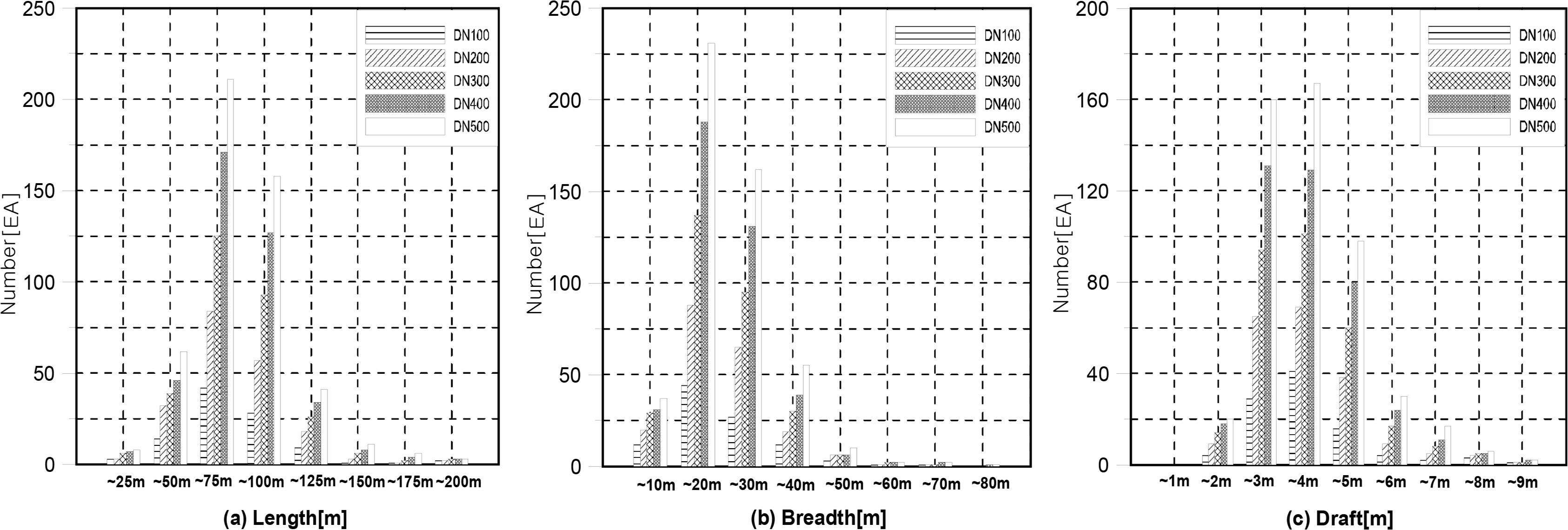
The number of pieces of data was changed from 100 to 500, in 100 intervals. Fig. 4 shows the distribution plot for each data. Here, the x-axis represents the length in Fig. 4(a), breadth in Fig. 4(b), and draft in Fig. 4(c), and the y-axis represents the number. The purpose of using similar data distributions by data number was to preprocess the data configurations before learning, as biased data can distort the accuracy of a learning model.
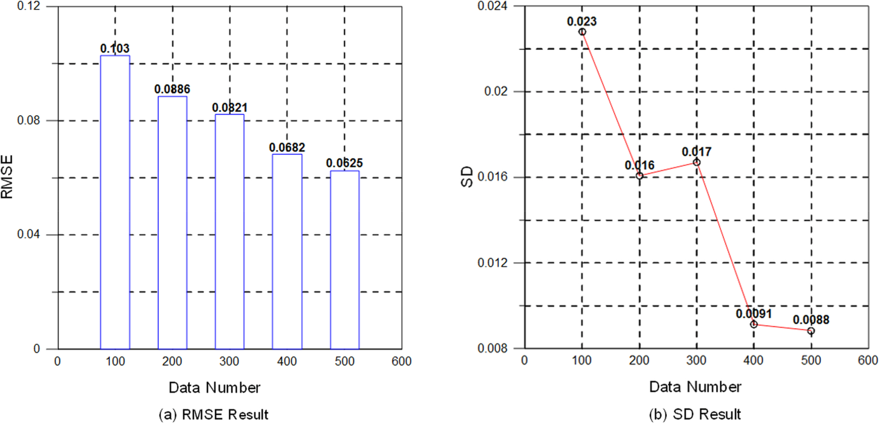
Fig. 5 shows the RMSE and SD values for 20 test data, according to the data number. In Fig. 5(a), it can be seen that the RMSE decreases with increasing data number. From Fig. 5(b), it can be seen that the variation of the accuracy also decreased.
Fig. 6 shows a graph with the seed number (0ŌĆō19) as the x-axis and RMSE as y-axis for the case of DN500_L2_NN(256,256). In this case, the data sets with the bottom 25% accuracies among the 20 seed numbers (3, 6, 8, 12, and 14) are indicated by red bars, whereas the data sets with the top 25% accuracies (0, 7, 11, 13, and 18) are indicated in black bars. Table 4 lists the values and means of the data with the bottom 25% and top 25% accuracies.
3.3.1 Seed number: 14
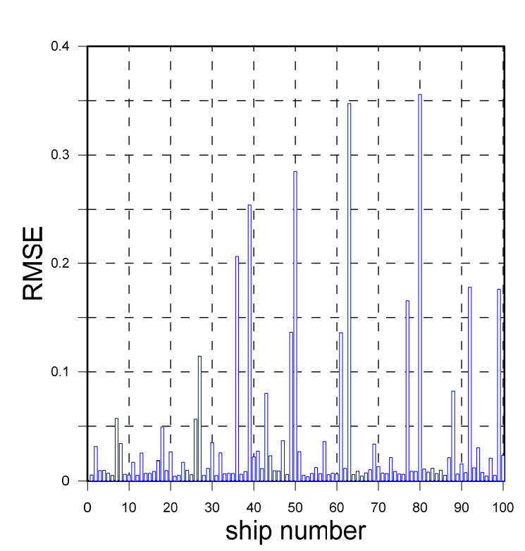
Seed number 14 is the data set with the highest RMSE, indicating that it has the lowest accuracy. However, the RMSE result of seed number 14 is derived as the mean RMSE for 100 ships, i.e., the test data. Considering that it is necessary to analyze the RMSE values for the 100 ships comprising the test data, a graph was generated for seed number 14, with the 100 ships of the test data on the x-axis, and the RMSE values of the ships on the y-axis (as shown in Fig. 7). A close examination of Fig. 7 reveals that the accuracy of the learning model for most of the ships is high, but the accuracy drops for some ships, owing to differences between the observed and predicted data.
Therefore, in this study, the RAOs of the bottom three ships and top three ships were compared as representative examples, and ships with a high RMSE were examined. For seed number 14, ships #21, #53, and #66 had low RMSEs, whereas ships #50, #63, and #80 had high RMSEs.
Fig. 8 shows graphs for comparing the observed and predicted data of the RAOs for ships #21, #53, and #66. Although there were slight differences between the observed and predicted data in a specific frequency range, the locations and sizes of the resonance points of the ships were predicted with high accuracy.
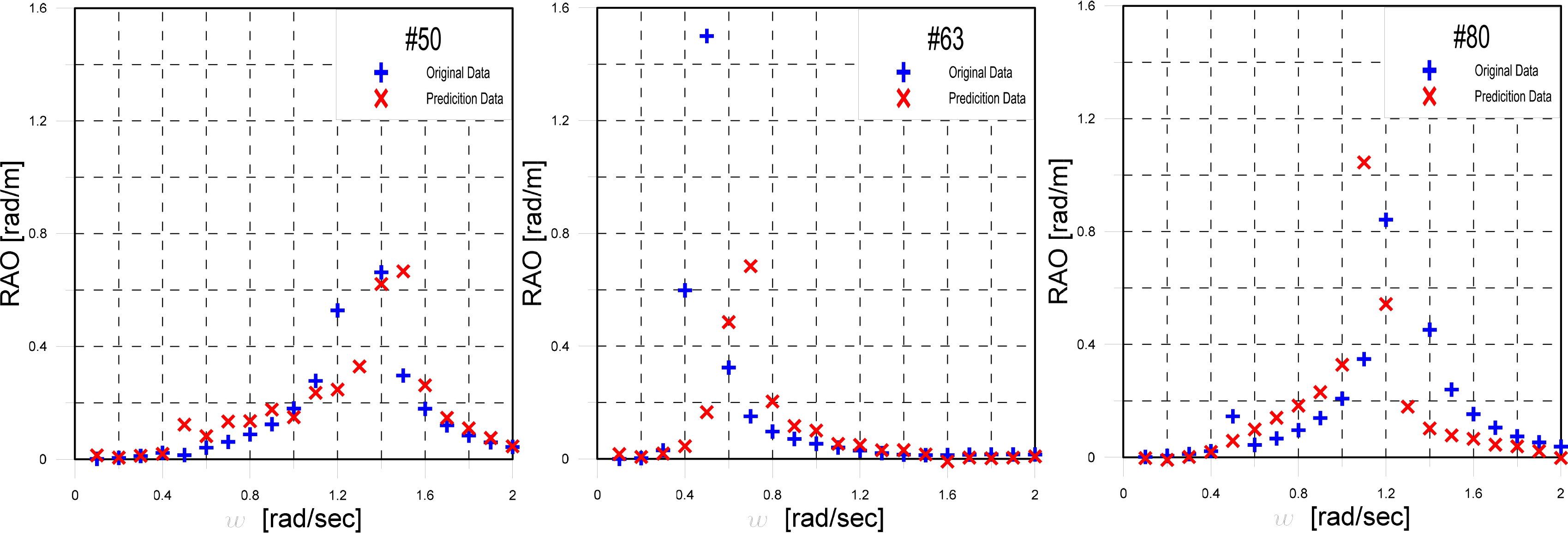
Fig. 9 shows graphs for comparing the observed and predicted data of the RAOs for ships #50, #63, and #80. It can be seen that ships #50, #63, and #80 have differences between the observed and predicted data at the locations of the resonance points. Furthermore, on the y-axis in Fig. 9, the size of the observation data at the resonance point is lower than 0.8 for ship #50, whereas the sizes at the resonance points of the observation data on the y-axis for ships #63 and #80 are approximately 1.2. This difference in the absolute values on the y-axis is another factor that increases the RMSE. Lastly, for ship #80, which has the lowest accuracy, there are differences in not only the location of the resonance point, but also in the size at the resonance point, as well as between the observed and predicted data over the entire frequency range.
3.3.2 Seed number: 18
Seed number 18 is the data set with the lowest RMSE, i.e., the data set showing the highest accuracy. The results were verified using the same method described for seed number 14 in Section 3.3.1. Fig. 10 shows a graph of 100 ships (the test data) on the x-axis, and the RMSE of each ship on the y-axis. A close examination of Fig. 10 reveals that although the accuracy of the learning model for most of the ships is high, the modelŌĆÖs accuracy for some ships decreases, owing to differences between the observed and predicted data.
As in Section 3.3.1, the RAOs of top three and bottom three ships were compared for seed number 18, and they were selected as the data for examining the reasons for high RMSEs. Ships #9, #56, and #69 from seed number 18 showed low RMSEs, whereas ships #11, #14, and #83 showed high RMSEs.
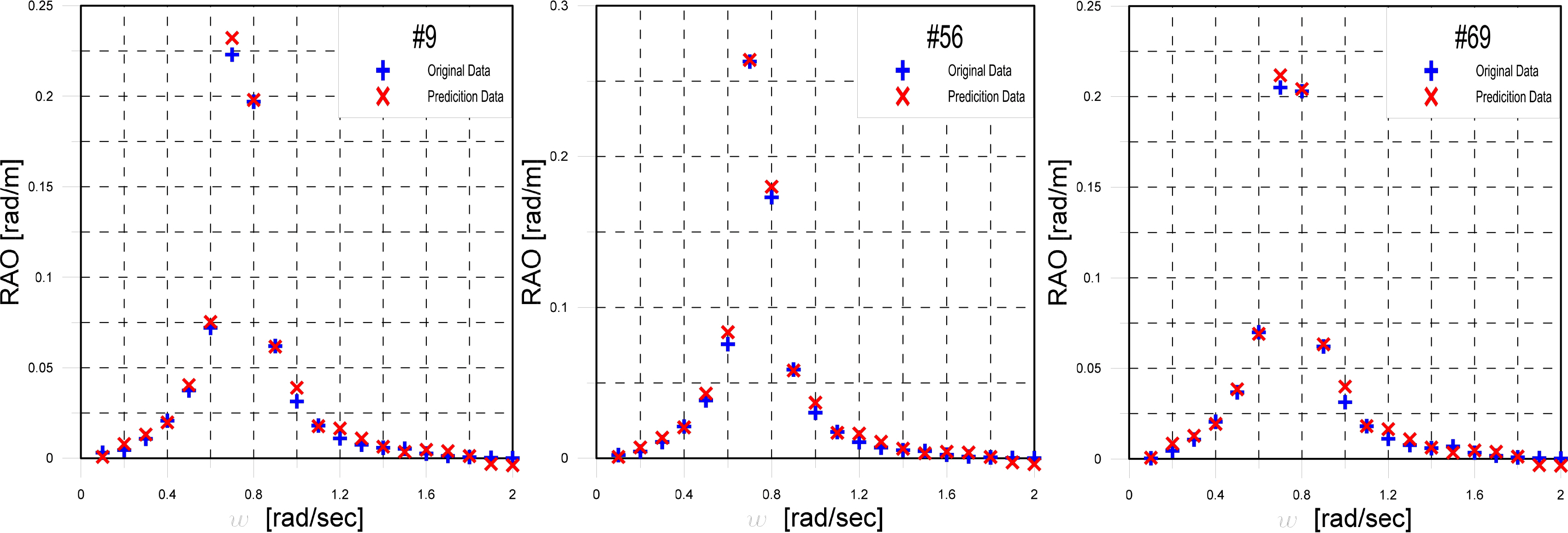
Fig. 11 shows graphs comparing the observed and predicted data of the RAOs for ships #9, #56, and #69. Similar to ships #21, #53, and #66 of the above-mentioned seed number 14, there were slight differences between the observed and predicted data in a specific frequency range, but the locations and sizes of the shipŌĆÖs resonance points were predicted with high accuracy.
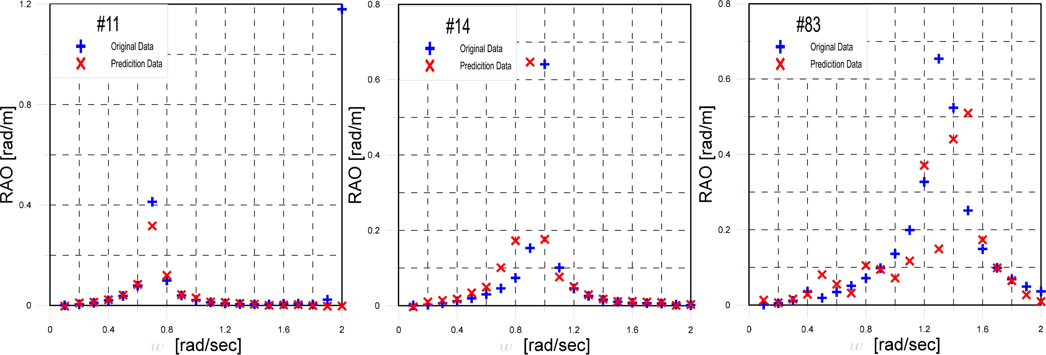
Fig. 12 shows graphs comparing the observed and predicted data for the RAOs of ships #11, #14, and #83. The RMSE of ship #11 was measured as high, as the observation data were abnormal at 2 rad/s. This is considered to be a noise generated when the high-frequency region was analyzed using the in-house code; the prediction data is considered to be the normal result. Thus, although ship #3 has the highest RMSE, data preprocessing for the abnormal result at 2 rad/s is expected to decrease the RMSE. In the case of ships #14 and #84, as mentioned above, a high RMSE is observed, owing to differences in not only the location of the resonance points, but also in the sizes at the resonance points, as well as between the observed and predicted data over the entire frequency range.
3.4 Learning Results with Different Numbers of Hidden Layers
The hidden layer calculates a weighted sum by receiving input values from the input layer and delivers this value to the output layer by applying it to an activation function. Regarding the number of hidden layers, one or two-layered neural networks are frequently used. Nevertheless, sometimes many hidden layers are required, owing to the purpose or complexity of the neural network. Therefore, to optimize the number of hidden layers in this study, the RMSE and SD values were obtained when increasing the number of hidden layers to two, three, and four.
Consequently, Fig. 13(a) shows a graph with the number of hidden layers on the x-axis and RMSE on the y-axis, and Fig. 13(b) shows a graph with the number of hidden layers on the x-axis and SD on the y-axis. An observation of these graphs reveals that when the number of hidden layers increased from two to three, the RMSE and SD increased slightly. When the number of hidden layers was four, the RMSE and SD increased sharply. Therefore, it was determined that two is the optimal number of hidden layers in this study.
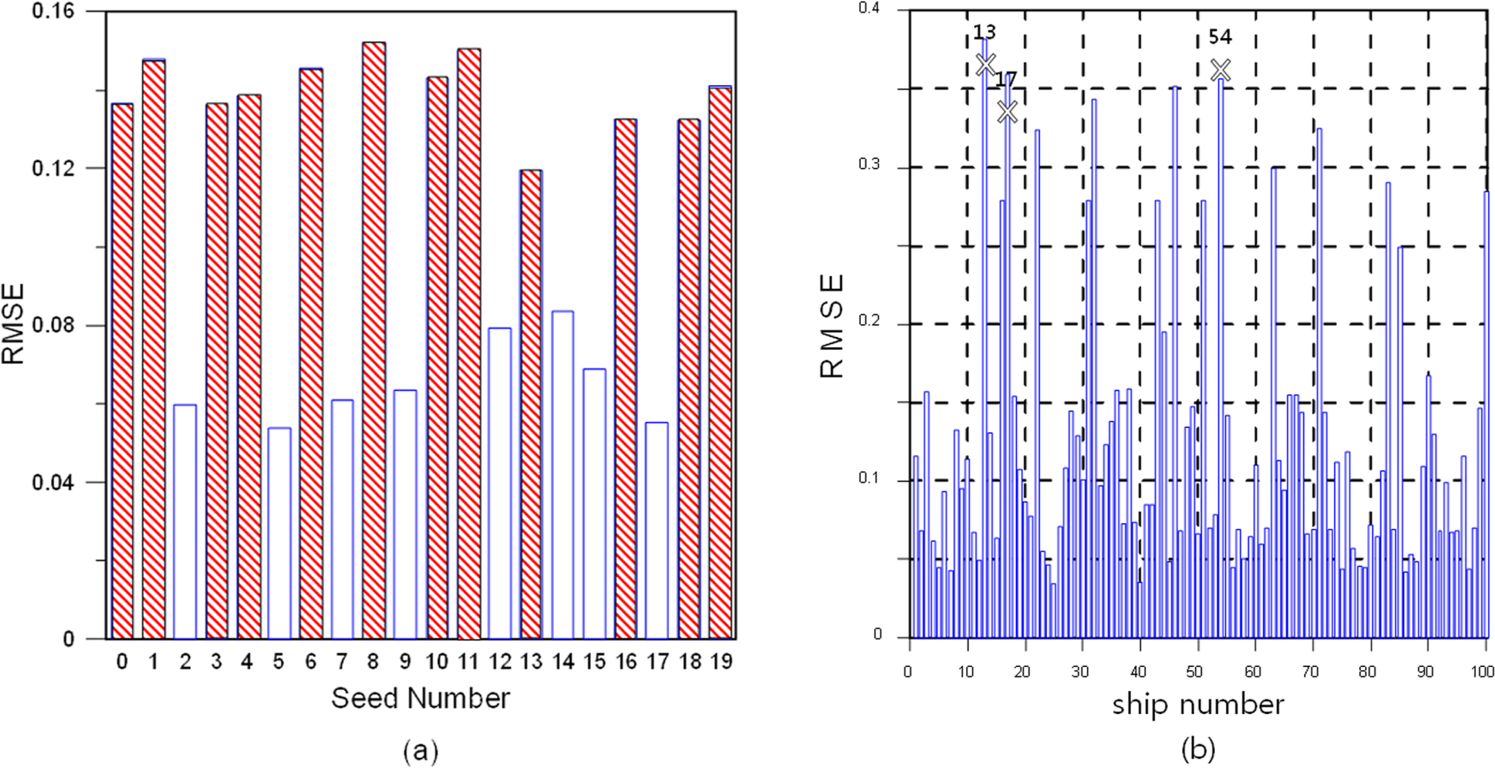
Fig. 14(a) shows a graph with the seed number on the x-axis and RMSE on the y-axis for DN500_L4_NN(256,256). The 12 RMSEs higher than the mean are marked by red slashes. Fig. 14(b) shows a graph of the RMSEs for 100 ships in seed number 8, which has high RMSEs. In Fig. 14(b), ships #13, #17, and #54, which have high RMSEs, are marked with an ŌĆśXŌĆÖ.
An observation of the prediction data for the three ships in Fig. 15 reveals that all of the ships have the same RAO, even though their specifications are different. Furthermore, a common phenomenon of predicting the same RAO is observed in the 12 seed numbers marked by red slashes, even though the 100 ships have different specifications. The cause of this phenomenon is considered to be the increased complexity of the system, owing to the increased number of hidden layers. In other words, it can be interpreted as a situation where the complexity increased, and the local minima was found in a certain part of the loss function instead of the global minima for the entire loss function, resulting in insufficient learning.
3.5 Learning Results with Different Numbers of Neurons in the Hidden Layer
In Sections 3.3 and 3.4, an intermediate conclusion was derived, i.e., that the optimal model is the case where there are data for 500 ships, and the number of hidden layer numbers is two. In this section, the learning results were analyzed according to different numbers of neurons in the hidden layer, to draw the final conclusions. During learning, there is difficulty in decision-making, as the number of neurons in the hidden layer depends on the userŌĆÖs experience, whereas the neuron numbers of the input and output layers are fixed. Therefore, in this section, the RMSEs of the learning model were compared, by changing the numbers of neurons in the hidden layer in the cases of DN500_L2.
A backward approach was used to configure these cases, in which the neural network was learned and tested while reducing the number of neurons in the hidden layer step-by-step. Table 5 outlines each case using the neural network structure. For cases 1, 2, and 4, the number of neurons in the learning model was selected randomly. The number of neurons for case 3 was selected by referring to a previous study (Stathakis, 2009). For cases 5 and 6, a rule of thumb from a previous study (Kim, 2017) was used.
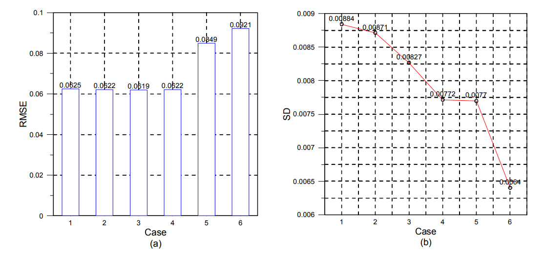
In Fig. 16(a), a tendency can be seen in that in general, as the number of neurons increased, the RMSE also increased. A close observation reveals that in case 3, the RMSE decreased somewhat, but the decrease was insignificant; moreover, in cases 5 and 6, the RMSEs increased sharply. In contrast, Fig. 16(b) shows that as the number of neurons decreased, the SD also decreased. In short, cases 1, 2, 3, and 4 have low RMSEs on average, but the fluctuations of the RMSE were larger than those of cases 5 and 6, depending on the assessment data. In contrast, cases 5 and 6 have relatively high RMSEs, but the fluctuations of those RMSEs are small. Cases 1, 2, and 3 cannot be the optimal model because their SDs are excessively large, although their RMSEs are similar to that of case 4. Furthermore, cases 5 and 6 have low accuracy regarding the prediction data owing to high RMSEs, although their SDs are smaller than that of case 4. Therefore, case 4 is considered to be the optimal model, as an appropriate compromise between the RMSE and SD.
3.6 Analysis of the Optimal Model Learning Result and Discussion
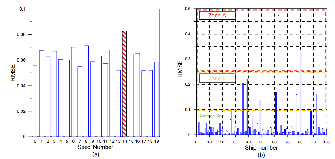
Fig. 17(a) shows a graph of the RMSE based on assessment data of the case DN500_L2_NN(100,100). In Section 3.5, the SD of case 4 was found to have small fluctuations. In addition, the RMSE values for each seed number comprising case 4 show that seed number 14 has a higher RMSE than those of the other test data.
Therefore, it is believed that an analysis of the test data for seed number 14 would improve the accuracy of the learning model, as well as the accuracy of learning results. Fig. 17(b) shows a graph of the RMSE for each ship in seed number 14. The results are analyzed by defining ŌĆ£Zone AŌĆØ for RMSE Ōēź 0.25 and Ōēż 0.5, ŌĆ£Zone BŌĆØ for RMSE Ōēź 0.0826 and < 0.25, and ŌĆ£Below AverageŌĆØ for RMSE < 0.0826. The RAOs were initially compared for ships #50, #63, and #80, which belong to Zone A, and then for ships #27, #77, and #92, which belong to Zone B.
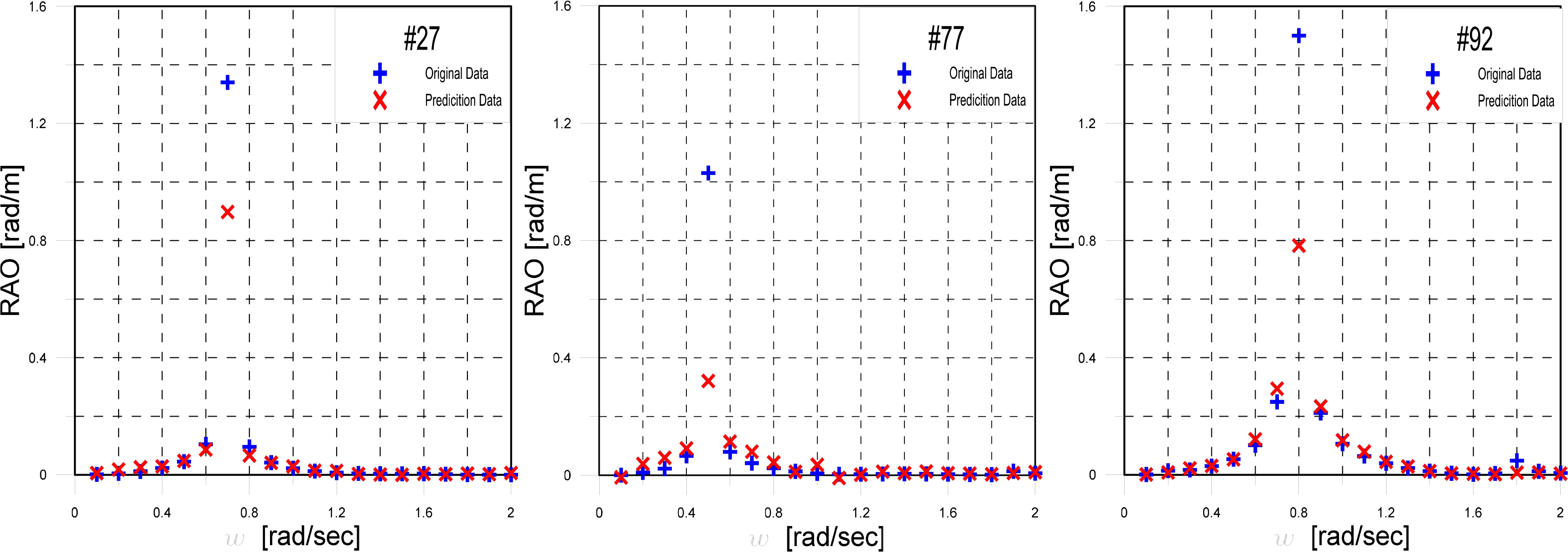
Fig. 18 shows a graph for comparing the RAOs of ships #27, #77, and #92, which belong to Zone B. These ships have somewhat lower accuracies than the mean, although higher than those of Zone A. Their RAO values over the entire frequency range are similar, and the location of the resonance is predicted with a high error. However, all three ships generated RMSEs, owing to differences in the sizes at the resonance point.
Fig. 19 shows a graph for comparing the RAOs of ships #50, #63, and #80, which belong to Zone A. Although they had the same general shape in the RAO, there were significant differences in the location and size of the resonance point, and between the observed and predicted data over the low- and high-frequency ranges. From Fig. 19, it can be concluded that the difference between the observed and predicted data is the main cause of the RMSE for the ships with high RMSEs in each seed number.
It is believed that understanding the distribution characteristics of the data set by obtaining the correlation(s) between the training and test data can improve the accuracy for ships with a high RMSE. Therefore, in Table 6, the correlation coefficients of the input variables (L, D, V, I44, C44, GMT) associated with the shipŌĆÖs breadth in the assessment and test data of seed number 14 were determined and ranked. For example, the breadth (B) and volume (V) of the training data showed a high positive correlation of 0.839, but in the assessment data, it was 0.737, i.e., a lower correlation than in the training data. Moreover, the correlations for features such as the coefficient of restitution (which is directly related to the location of the resonance point) were different. This indicates that the low accuracy was caused by the differences between the trends of the training and assessment data.
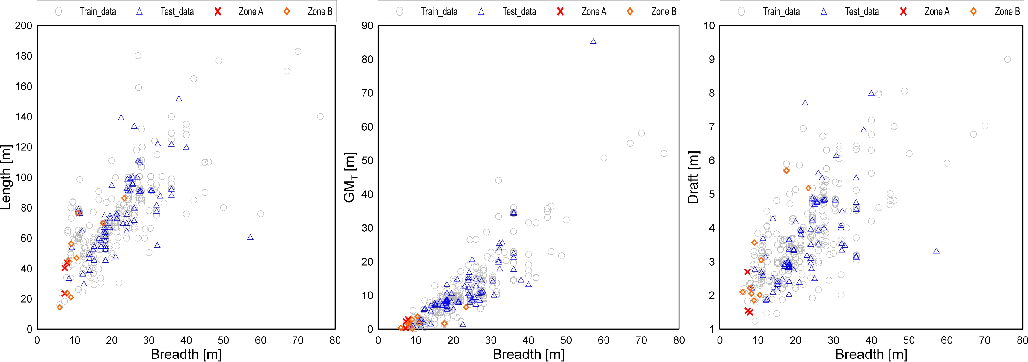
Fig. 20 shows a scatter plots where the x-axis is set as the shipŌĆÖs breadth, and the y-axis is set as the length, draft, and transverse metacenter height. They shows the training data (gray circle), test data (blue circle), Zone A with high RMSEs (red cross mark), and Zone B with medium accuracy (orange diamond), as used in this study. Typically, when one specification of a ship (such as length) is determined, the other specifications, e.g., breadth and draft, have specific ranges. This means that the specifications of ships have certain correlations with one another, and these correlations can be also seen in the scatter plots.
The scatter plot in Fig. 20 indicates that the data are concentrated in a specific section, and that ships having a high RMSE (Zone A) are located in an area with a low data density. In other words, ships with specifications that have not been sufficiently trained have low data accuracy. Figs. 18ŌĆō19 show that while the accuracy was somewhat insufficient for Zone A, the overall RAO trend for the ships belonging to Zone B was predicted, even though the RMSE was high. Furthermore, considering that only a difference in the size at the resonance point caused an RMSE for certain ships, it can be said that there are cases where the prediction data of the RAO is reliable, even in a region with low data density.
4. Conclusions
This study was conducted to predict the roll RAO of barge-type ships using machine learning. The input variables (L, B, D, V, k44, I44, C44, GMT) were generated using the specifications of 500 barge-type ships registered with classification societies. In addition, the values for the roll RAO were obtained by simulating the 500 ships using an in-house code based on a 3D singularity distribution method, and the features and RAOs of the data sets were configured. Finally, the data were composed with the RAOs in the range of 0.1ŌĆō2.0 rad/s, according to the major specifications of the barge-type ships. For the learning model, an ANN was created using PythonŌĆÖs TensorFlow, and a DNN technique with two or more hidden layers was used. The accuracy of the learning results was determined by changing the number of datapoints, number of hidden layers, and node numbers in the hidden layer. The RMSE, SD, correlation coefficient, and scatter plot were used as accuracy indices. When the RMSE and SD were considered together, the optimal results were obtained in case 4 [DN500_L2_NN (100,100)]. Finally, the shortcomings of the learning model and possible improvements were examined through an analysis of the accuracy of Case 4.
The conclusions of this study can be summarized as follows.
(1) The accuracy of the learning model can differ depending on the combination of training and test data. Therefore, the reliability of the learning results can be improved by collecting sufficient data.
(2) The accuracy increases when there are more high-quality data following the statistical distribution.
(3) Using many hidden layers can lower the accuracy, by increasing the complexity of the neural network model.
(4) The optimal model in this study is DN500_L2_NN(100,100).
(5) There are three main factors causing low accuracy in RAO prediction:
- Failure to accurately predict the location of the resonance point;
- An increase of RMSE owing to a difference in size between the observed and predicted data at the resonance point, and
- Differences between the observed and predicted data over the entire frequency range.
(6) The scatter plot showed that ships with low accuracy are located in an area with a low data density.
(7) This study did not consider various data on the centers of gravity of the barge ships, which involves practical difficulties. Therefore, a study considering various centers of gravity should be conducted.


 #3
#3 #0
#0


