


1. Introduction
Maneuverability is one of the most important performances of a marine vehicle which plays a vital key in the safety of navigation and efficient service. Unlike the floating vehicle, the submarine must be controlled in the six degrees of freedom. Hence, the configuration of control surfaces is also more complex to meet the demand of its controllability. Therefore, assessment of maneuverability of the submarine with control surfaces is required as well. In order to evaluate the maneuvering characteristics at the design stage, it is necessary to predict hydrodynamic force and moment acting on the vehicle in various modes of motion. It can be categorized that there are available four methods for estimating the hydrodynamics. Semi-empirical methods have been used for calculating the hydrodynamic derivatives, but these have just simple form and deal with only main design particulars of the submarine(Mackay, 2007). In addition, the panel method was developed to predict the hydrodynamic characteristics of the underwater vehicle. Nevertheless, this method did not take into account the effect of viscosity, so it could deal with only added mass and added moment of inertia(Iskender et al., 1997). Captive model tests are considered as the most accurate method to determine all linear and nonlinear hydrodynamic derivatives used for mathematical modeling of hydrodynamic force and moment(Park et al., 2017; Han et al., 2017). However, it also has some disadvantages such as the limitation of facilities, the high cost of performance, and the scale effects.
On the other hand, Computational fluid dynamics(CFD) methods are becoming the alternative solution for compromising the disadvantages of the other methods. It not only includes the viscous effects but also can model the captive model tests virtually with good accuracy and economy as well. There are three main approaches to simulate turbulent flow over the submarine, which are Direct numerical simulation(DNS), Large eddy simulation(LES), and Reynolds-averaged Navier-Stokes(RANS). DNS is the most accurate of approaches as it numerically solved Navier-Stokes equations without any turbulence model, but it requires enormous computational resources. The LES or hybrid LES-RANS approach are computed directly and only small scale motions are modeled. It is more accurate than the RANS approach since the large eddies are captured in full detail directly. However, these approaches are many times more computational expense than RANS approach. The RANS is the most common approach to turbulence modeling using the Reynolds averaging procedure. Nonetheless, it gives bad results when there is swirl or streamline curvature.
Regarding the use of RANS calculation in the design of submarine, Toxopeus(2008) and Zeng and Zhu(2010) demonstrated that RANS-based simulation could be used to predict the hydrodynamics of the scaled DARPA SUBOFF submarine in forward and oblique motions at small drift angle. In addition, Pan et al.(2012) proposed an approach for simulating the small drift motion and the harmonic motion of the same submarine with full appendage using the unsteady RANS-based simulation and the dynamic mesh technique. To solve the rotational motion by CFD method, Wu et al.(2015) employed the hybrid reference frames method to model the circular motion of the DARPA SUBOFF submarine. These researches show that the results of the RANS-based simulation are in good agreement with the experimental data. However, the simulations were mainly carried out for the scaled model with a few motion modes.
In the present paper, the RANS-based simulation for a full-scale submarine with appendages is done at straight motion, oblique motion, and rotational motion for both single mode and combined mode in the horizontal plane and vertical plane. The obtained force and moment of the simulations are then analyzed and non-dimensional hydrodynamic derivatives are estimated using least square method for maneuvering assessment in the further study.
2. Case study
2.1 Objective
The submarine shape in this paper is modeled following the outline of the submarine type with 85.0 m long, 7.7 m wide, and 6.7 m depth. Conning tower and rudder are created from NACA0020 profile, and the NACA0018 profile is used for the remained control surfaces. Fig. 1 shows the definition of body-fixed coordinate system and outline drawing of the submarine which is used in this study.
2.2 Test conditions
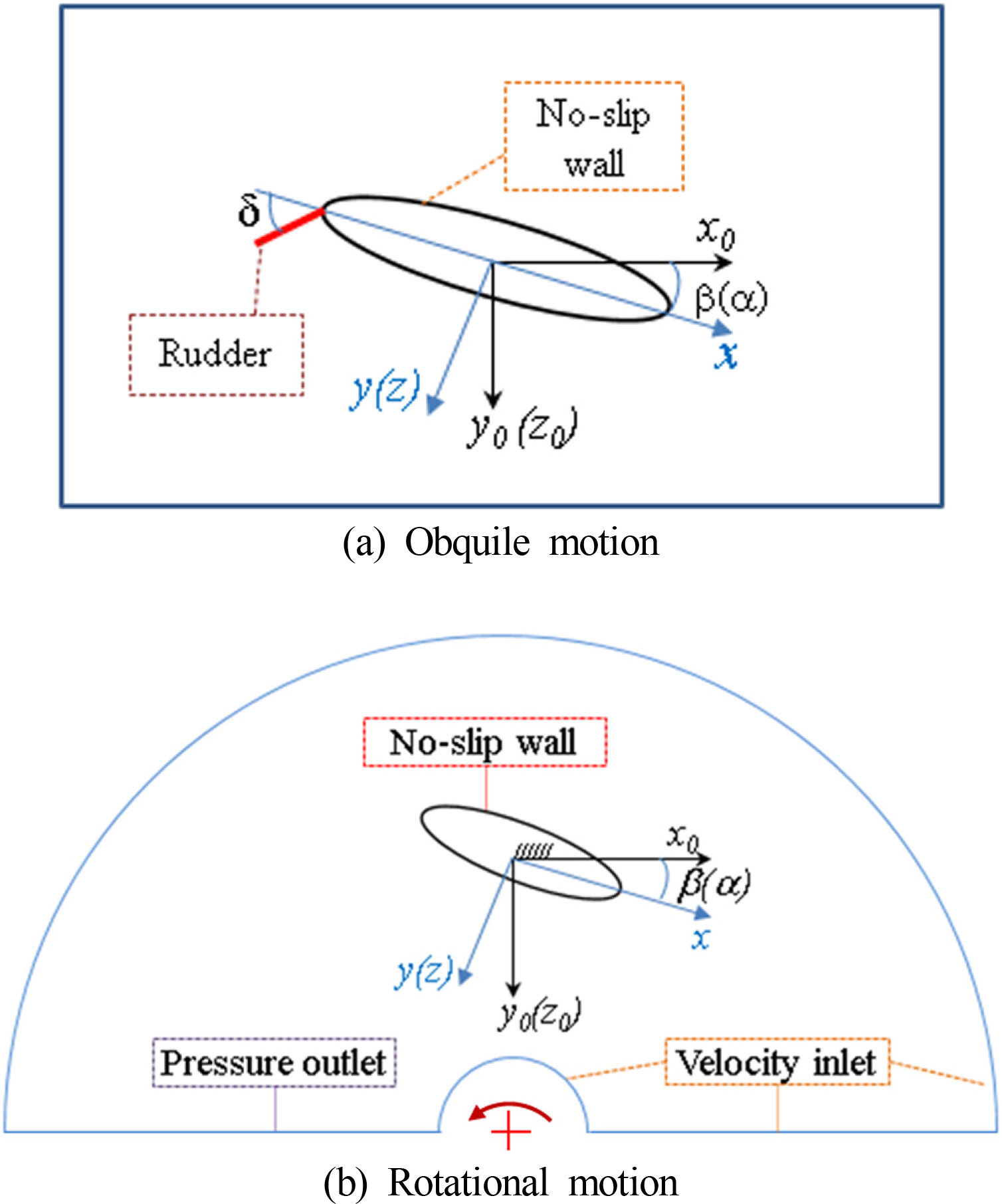
In order to estimate the hydrodynamic derivatives, the virtual captive model tests of the vehicle are implemented for a series of motion modes at Reynolds number of 8.7099602E+08. The definition of the submarine motions is described in Fig. 2, where α, β, δ and ω are called the angle of attack(AOA), drift angle, and deflection of control surfaces, and rotational velocity, respectively. Fig. 2(a) shows the definitions of straight running(α, β, δ =0), oblique(α or β ≠ 0, δ = 0), and the deflection of control surfaces(α, β = 0, δ ≠ 0). The circular motion(α, β = 0) and combined circular motion(α, β ≠ 0) are illustrated in Fig. 2(b). Following the International towing tank conference(ITTC) recommendations on Captive Model Tests Procedure(ITTC, 2014), the computing conditions of these cases are selected as shown in Table 1.
The velocities and hydrodynamic force and moment obtained from the simulations are presented in the dimensionless form as follows,
where u, v and w are the velocity components along x, y and z-axes, respectively. q and r are the angular velocities of y and z axes. X, Y and Z are the hydrodynamic forces along x, y and z-axes, respectively. M and N are hydrodynamic moments about y and z-axes.
2.3 Numerical modeling
The rectangular domain and cylindrical domain covering the submarine are generated for simulating the straight and oblique motion, and the circular motion, respectively. Its dimensions are chosen to be able to eliminate the effects of wall boundaries as well as reverse flow at the inlet and outlet flow conditions. Dimensions of the rectangular domain are 5 L in length, 4 L in width, and 3 L in height. These are 0.2 L, 5 L, and 3 L for inner radius, outer radius, and thickness of the cylindrical domain. In addition, physical conditions are applied for the boundary of the domain. The front face and back face are correspondingly assigned to velocity inlet and pressure outlet. Slip condition is set for the side walls and the no-slip condition is specified for the appendages and hull surfaces. The top face and bottom face of the domain is considered as slip wall conditions.
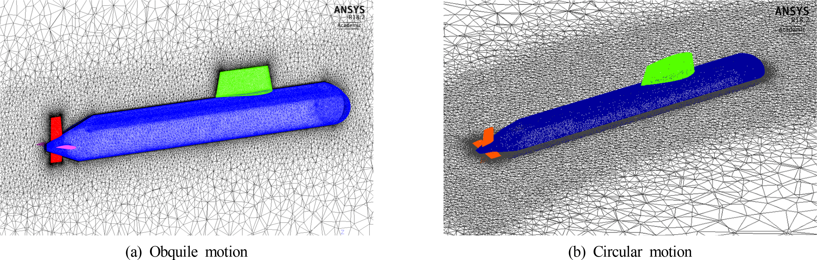
The fluid domain is then discretized in a number of tetrahedral elements for the numerical process. Prism layer is used for modeling boundary layer of fluid flow surrounding the hull. The height of the first element next to the body’s wall is created to satisfy y+ value of the boundary layer. The value of y+ can be set about 3,000-5,000 for Re = 1.0E+9(Oh and Kang, 1992), and the boundary thickness of submarine in the trial(William, 1974) is in fair agreement with the empirical relation of Granville. Using these two references, the estimated first grid height is 9.0 mm corresponding to y+ of 2,500. Fig. 3 shows the mesh of submarine in the fluid domain.
The ANSYS FLUENT software is applied for simulating the single motion and the coupled motion of the submarine in steady state. An incompressible RANS solver is opted for modeling fluid flow in these cases. According to ITTC Practical Guidelines for Ship CFD Applications(ITTC, 2011), the two-equation models have shown to be able to give an accurate prediction in ship hydrodynamics. Hence, the realizable k-epsilon turbulence model is chosen for modeling fluid flow around the submarine. Also, the second order upwind scheme is used for determining face values from interpolation of cell center values with the good accuracy and robust. Semi-implicit pressure link equations(SIMPLE) algorithm is employed to obtain pressure field and face flux by solving the momentum equation iteratively(ANSYS, 2017). Evaluation of the gradients and derivatives is done using the least square cell-based method.
The straight and oblique motions of the submarine are simulated in stationary reference frame while the steady circular motions and combined motions are carried out in moving reference frame. Following the method(ANSYS, 2017), the relative velocity vectors are defined as follows,
where υr stands for the fluid relative velocity, υ denotes the fluid absolute velocity, ur is the velocity of the moving coordinate system including translational velocity υt and rotational velocity ω. R is the radius of the motion.
3. Results and discussions
The full-scale model runs steadily with the design speed of 20 knots (10.29 m/s). After the solution is converged at 10-5, the hydrodynamic forces and moments acting on the ship will be obtained. It is then nondimensionalized and fitted with polynomial functions for determining the dimensionless derivatives. The velocity-dependent derivatives can be taken from straight and oblique motions while rotary derivatives are extracted from the circular motion. The cross-coupled derivatives are attained in the combined motion simulation. These derivatives are used to establish the mathematical model of the hydrodynamic force and moment acting on the hull(HD) and control surfaces(C). According to Feldman(1979), the hydrodynamic forces and moments are mathematically modeled as follows:
Axial force:
(4)
Lateral force:
(5)
Normal force :
(6)
Roll moment:
(7)
Pitch moment:
(8)
Yaw moment:
(9)
where eg. X u ˙ ' = ∂ X ' ∂ u ˙ K p ˙ ' = ∂ K ' ∂ p ˙ X q q ' = ∂ 2 X ' ∂ q 2 K p ' = ∂ 2 K ' ∂ p X ν r ' = ∂ 2 X ' ∂ ν ∂ r K w p ' = ∂ 2 K ' ∂ w ∂ p X δ r δ r ' = ∂ 2 X ' ∂ δ r 2 K δ r ' = ∂ 2 K ' ∂ δ r
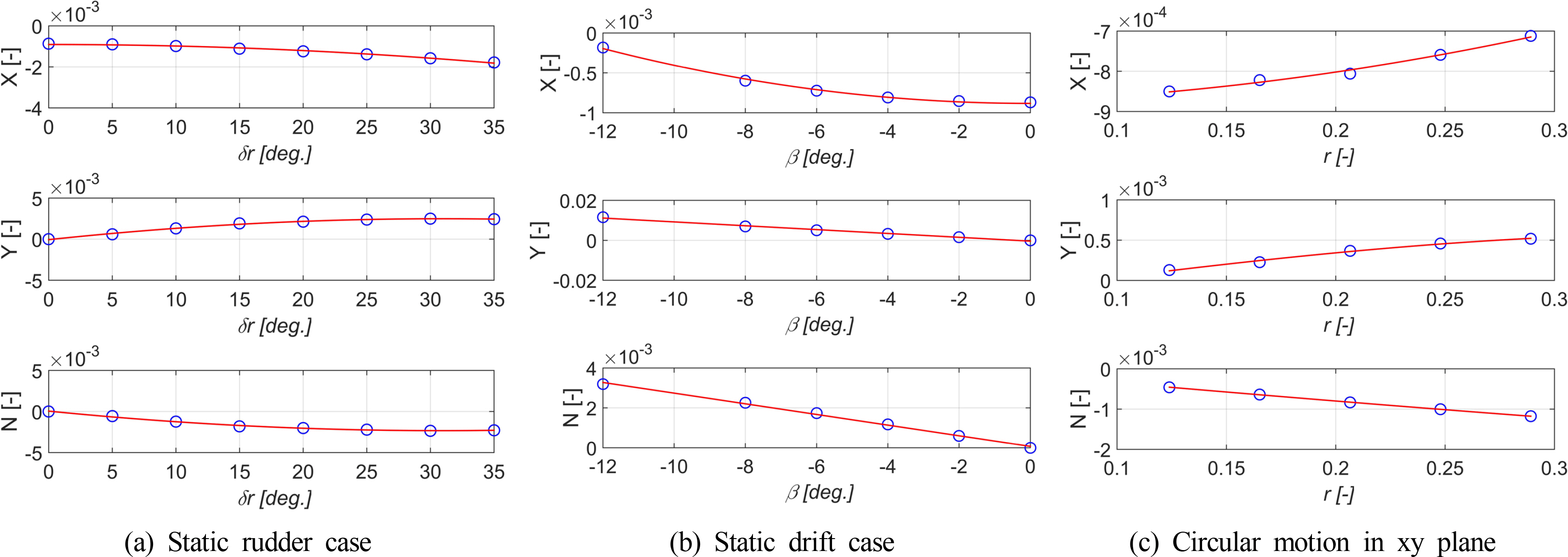
The ship is symmetrical about the vertical center plane, the calculations are implemented in the positive range of drift angles and rudder angles. Fig. 4 shows the forces and moments acting on the ship and rudder in cases of the static rudder, drift motion, and circular motion(CM) in the horizontal plane. The hydrodynamic force acting on the ship in cases of stern stabilizer, angle of attack, and circular motion in the vertical plane is shown in the Fig. 5. It can be seen that the forces acting on the submarine in case of positive attack angle are greater than the one for the negative side. The discrepancy between the two case decreases with increasing of the attack angle and it might be caused by the asymmetry in the vertical plane of the body as well as the effect of the lifting surface at the stern.
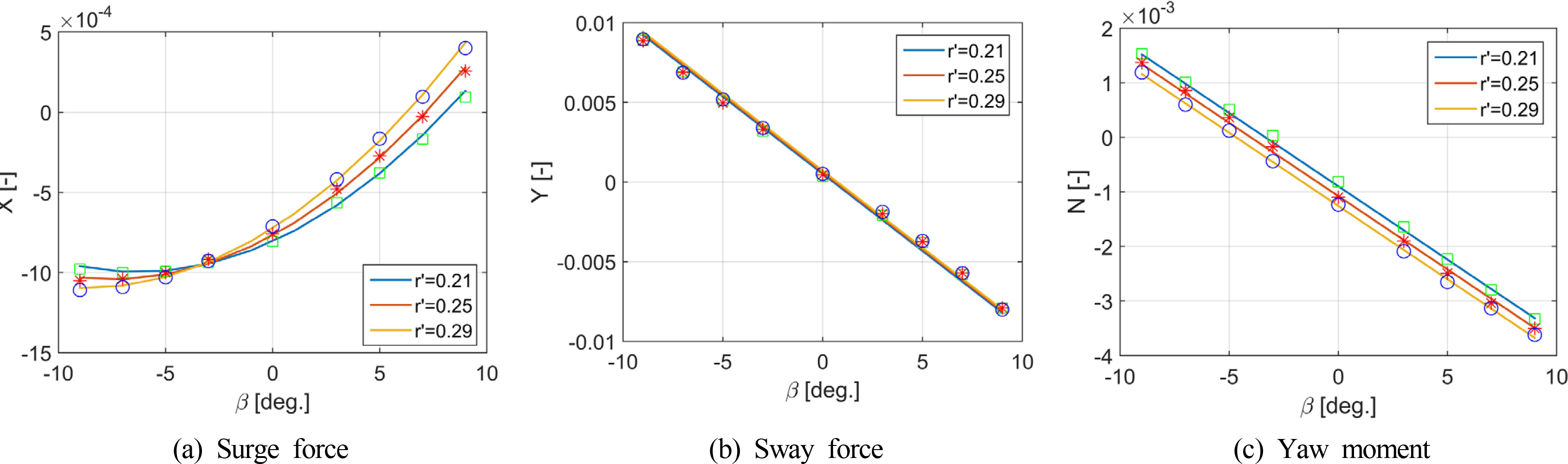
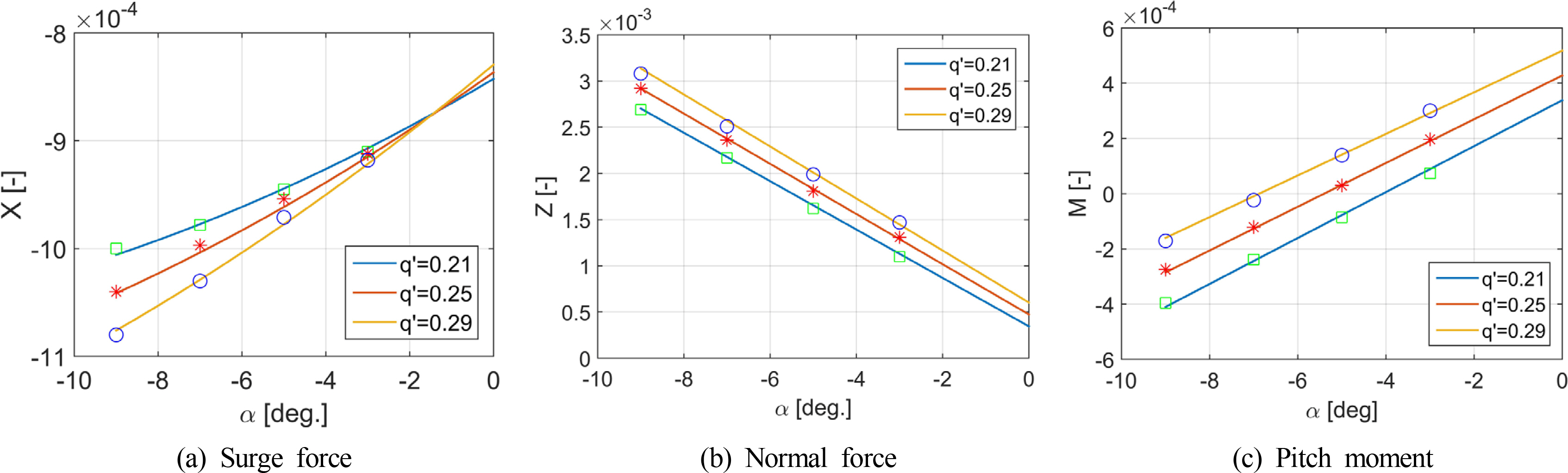
The coupled derivatives are determined from the combined motion by subtracting forces and moments acting on the ship in the single motions from the forces and moments acting on the ship in the combined motion. The residual forces and moments are approximated using the least square method. However, the results of the combined drift-circular motion show that linear function of sway velocity and yaw rate is enough to represent the variation of sway force and yaw moment. On the other hand, the hydrodynamic forces of the combined angle of attack and circular motion result in two coupled derivatives. Figs. 6-7 describe the force and moment acting on the submarine and fitting curves in these two cases. The hydrodynamic derivatives obtained from the simulation in this study are listed in Table 2.
Flow pattern around the sumarine is extracted to visualize flow characteristics during its operation. Fig. 8 illustrates contours of velocity magnitude in four cross sections located at fore and aft of the submarine. It can be seen that there is a development of vortex flow behind the conning tower. It becomes stronger as the vorticity sheds from the conning tower to the stern. The vortex generates the asymmetric forces acting on the submarine which afftects diving motion.
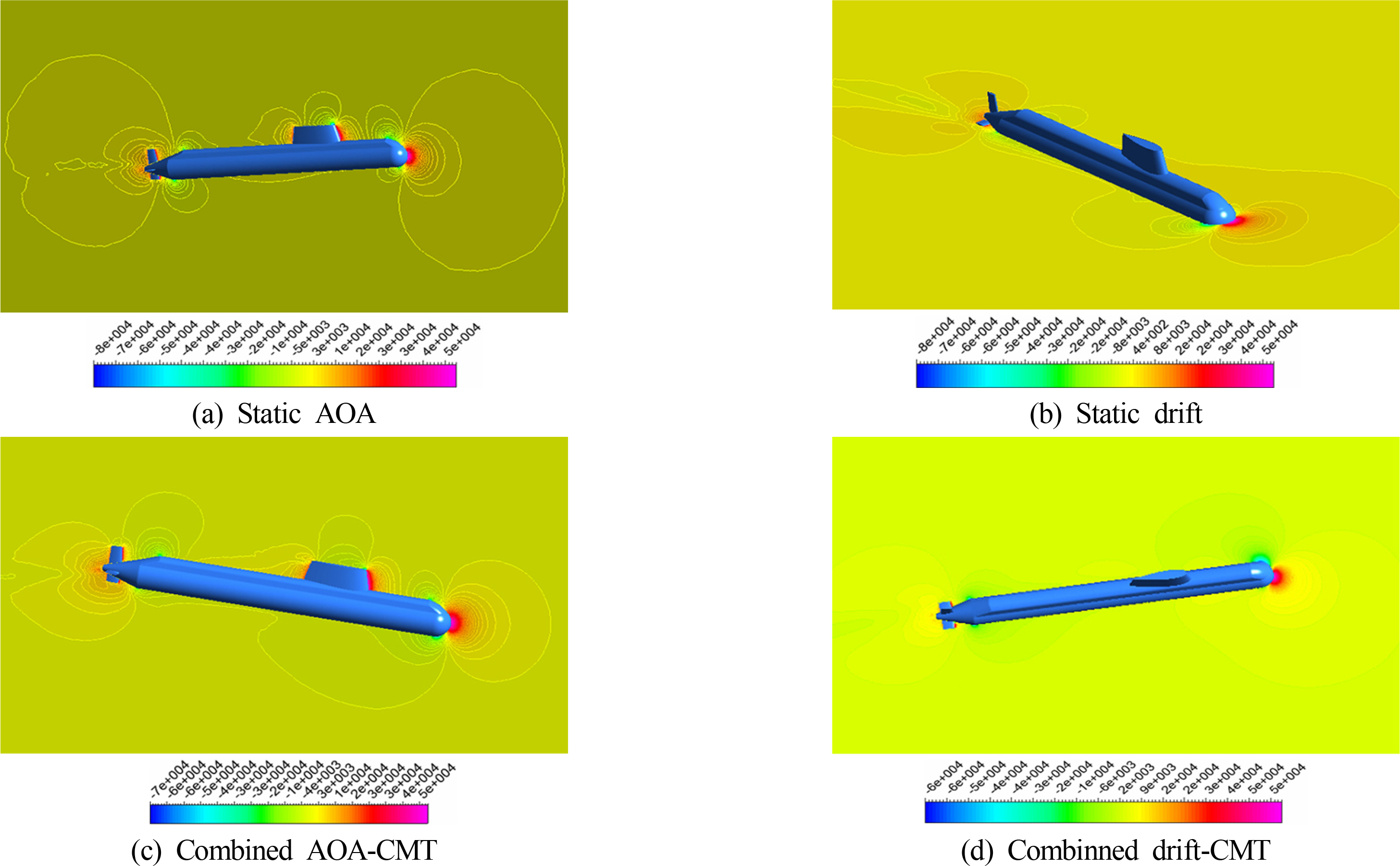
Fig. 9 shows the pressure fields of the vehicle when it travels in the angle of attack, drift, the combined angle of attack and circular, and combined drift and circular motions. The slices in the center plane and horizontal plane are colored by pressure distribution of flow around the hull and appendage. It is observed that the oblique and the combined motion cause asymmetry pressure field which leads to sway force, heave force, pitch moment, and yaw moment.
4. Conclusions
In this study, CFD RANS-based simulation of a full-scale submarine has been implemented when it runs straightly and rotationally. The straight motion and obquile motion is simulated in the stationary reference frame and the circular motion is modeled using the moving reference frame. The simulation results are fitted to curves and surfaces using the least square method. As the results, the velocity-dependent derivatives, rotary-dependent derivatives, and cross-coupled derivatives are estimated. These derivatives may be used to confirm the submarine’s maneuverability in its preliminary design. In the future, the simulation results will be verified with the experimental results.