A submerged body with varied control inputs can execute large drift angles and large angles of attack, as well as basic control such as straight movement and turning. The objective of this study is to analyze the dynamic characteristics of a submerged body comprising six thrusters and six control planes, which is capable of a large drift angle and angle of attack motion. Virtual captive model tests via were analyzed via computational fluid dynamics (CFD) to determine the dynamic characteristics of the submerged body. A test matrix of virtual captive model tests specialized for large-angle motion was established. Based on this test matrix, virtual captive model tests were performed with a drift angle and angle of attack of approximately 30° and 90°, respectively. The characteristics of the hydrodynamic force acting on the horizontal and vertical surfaces of the submerged body were analyzed under the large-angle motion condition, and a model representing this hydrodynamic force was established. In addition, maneuvering simulation was performed to evaluate the standard maneuverability and dynamic characteristics of large-angle motion. Considering the shape characteristics of the submerged body, we attempt to verify the feasibility of the analysis results by analyzing the characteristics of the hydrodynamic force when the large-angle motion occurred.

Keywords: Submerged body; Computational fluid dynamics; Large angle of attack; Virtual captive model tests; Maneuvering simulation

1. Introduction

A submerged body refers to all vehicles operated in water, such as a remotely operated vehicles (ROVs), autonomous underwater vehicles (AUVs), underwater weapons, and submarines (Kim et al., 2012; Park et al., 2015). Different types of submerged bodies serve varying purposes in military or commercial applications. Because submerged bodies have distinct operational purposes, their dynamic characteristics must reflect their operational purpose, and their shapes must be designed to satisfy the required dynamic characteristics accordingly. Therefore, a submerged body must be developed with a suitable performance for each task and utilization (Jeon et al., 2017). In particular, it is difficult to monitor the state of a small submerged body with the human eye because it is often remotely controlled or autonomously driven, unlike vessels manned by humans. Therefore, the maneuverability of such a submerged body needs to be sufficiently examined during the design stage to ensure the adoption of an appropriate controller.

Studies based on experimental and analytical methods have been actively conducted on estimating the maneuverability of a submerged body. The most accurate maneuverability analysis in the design stage involves modeling the external force of maneuvering equations of motion that reflect the motion range and operational purpose of a submerged body and estimating the external force model coefficients by performing a captive model test in a towing tank. Bae and Sohn (2009) conducted a static test including a resistance test in a circular water channel for Manta-type unmanned underwater vehicles. The maneuvering equation of motion with six degrees of freedom for Manta-type unmanned underwater vehicles was established by combining certain damping coefficients determined via a static test with added mass and damping coefficients estimated theoretically, and then, maneuverability was analyzed. Kim et al. (2012) conducted a captive model test by installing a submerged body model in a large-scale controlled computerized planar motion carriage. In addition to stability analysis, resistance, static drift, static angle of attack, horizontal and vertical turning, and combined tests were performed to estimate a damping coefficient, excluding the added mass coefficient. Jung et al. (2014) estimated added mass and damping coefficients by performing a vertical planar motion mechanism test in a linear towing tank for an autonomous underwater glider. In addition, they modeled the equation of motion based on the estimated coefficients to be adopted as the plant model for a control simulation. Owing to the cylindrical shape of most submerged bodies, the roll hydrodynamic damping moment is relatively small, and it triggers a large rolling motion at a high speed if the rolling motion is not properly controlled. To estimate a rolling motion of a sensitive submerged body, Park et al. (2015) conducted a coning motion test to estimate the hydrodynamic derivative, which is related to rolling motion, and proposed a different coning motion test method. The aforementioned model test cases were conducted for submerged bodies with slender shapes, under the assumption that the drift angle and angle of attack were not large at the design speed; hence, additional research is required to reflect a large angle of attack motion.

Estimating the maneuverability of a submerged body via analytical methods can be divided into two categories. The simplest approach adopts an empirical formula. Yeo et al. (2006) deduced the effect of design factors on the stability of a submarine based on an empirical formula that assumes that the main body is a lift force generator, which they substituted with an equivalent wing. Jeon et al. (2017) analyzed the effects of shape design factors on the maneuverability of a submerged body. However, an empirical formula was used to establish a plant model for designing a controller and estimating a linear stability coefficient for stability analysis. Simulating the large attack angle motion and slow motion is limited because a nonlinear coefficient cannot be estimated. The other approach involves conducting virtual captive model tests based on computational fluid dynamics (CFD). Recently, estimating hydrodynamic derivatives by performing a CFD in the same condition as a captive model test conducted in a tank has been widely adopted, and the accuracy results are similar to that of a model test. Sung and Park (2015) conducted a CFD-based virtual captive model test for open merchant vessels, KCS (KRISO Container Ship) and KVLCC (KRISO Very Large Crude-oil Carrier) 1&2, and compared the accuracy with the free running model test results. In terms of accuracy, They produced outstanding results. Nguyen et al. (2018) calculated the hydrodynamic force acting on a full scale submarine using a CFD analysis based on the Reynolds-averaged Navier–Stokes equations (RANS), and estimated damping coefficients. Cho et al. (2020) performed a virtual captive model test using CFD for submarines equipped with an X-rudder and deduced results similar to an experimental outcome.

In general, a large attack angle motion needs to be considered in a case when a vessel is operated at a low speed when berthing at a port (Takashina, 1986; Yoon and Kim, 2005), or when lateral and vertical movements are free, such as in ROVs (Jeon et al., 2016). In this study, we analyze the dynamic characteristics of a submerged body equipped with six thrusters and six control panels. A submerged body with various control inputs has relatively more free motions than a slender-type submerged body comprising a rudder attached in the rear part, elevator, and thruster. Specifically, motions in large drift angles and large angles of attack are possible. Because the motions are in large drift angles and large angles of attack, the motion range needs to be set broadly to accurately estimate the hydrodynamic force in the analysis.

Maneuverability can be directly investigated if a virtual free-running model test is conducted using CFD; however, it requires a significant amount of computation resources, and the maneuvering equation of motion, which is a plant model used for designing controllers, cannot be determined. Therefore, a virtual captive model test was performed in this study via CFD analysis to analyze the dynamic characteristics of a submerged body with a large angle of attack motion. This method is more advantageous than a model test in terms of time and cost, and it is also more advantageous than a water vessel in terms of computation time because computation is performed in water instead of on a free surface.

Most previous studies first established a maneuvering mathematical model and then estimated maneuvering coefficients comprising the mathematic model in their analyses. However, it is challenging to establish a mathematical model when the force tendencies are not thoroughly examined, the correlation between forces and motions is difficult to predict, and the data available on the submerged body are insufficient. Therefore, this study first examined the tendency of forces by establishing the conditions of a virtual captive model test in which hydrodynamic forces including large angles of attack motion were estimated and then modeled the correlation between forces and motions.

2. Coordinate System and Test Conditions

2.1 Coordinate System

Fig. 1 presents a coordinate system comprising the Earth-fixed coordinate for expressing the motion trajectory, orientation angle, and a body-fixed coordinate for defining the equation of motion and external forces acting on a submerged body. All the symbols used in the equation of motion and coordinate system are in accordance with the symbolic notation defined by Fossen (2011).

Fig. 1

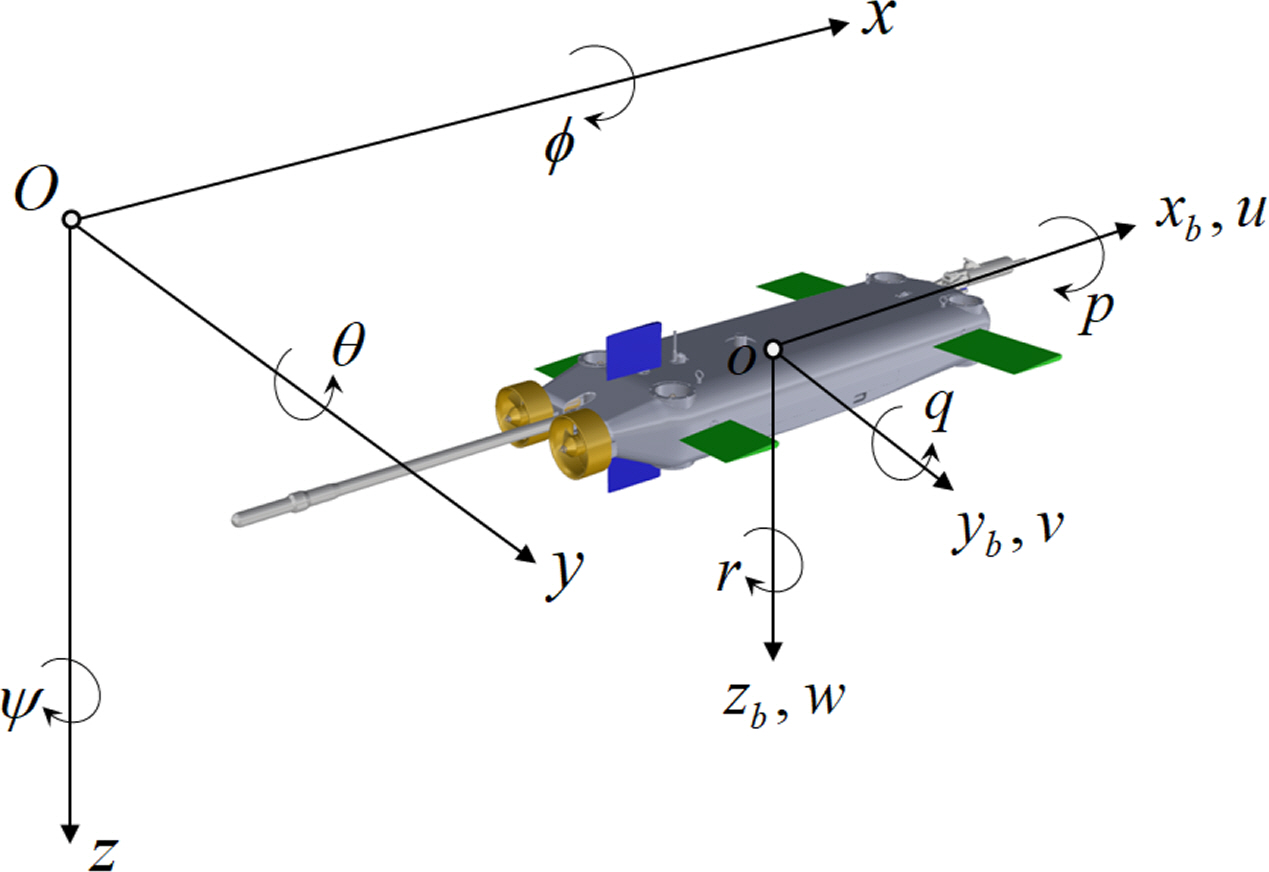
Coordinate systems

2.2 Subject Submerged Body

Fig. 2 shows that the subject submerged body is equipped with two main thrusters in the rear part and four auxiliary thrusters for adjusting the depth, including a rudder for controlling directions, a bow plane for controlling depth, and a rear elevator. Here, six control inputs generate thrust and rudder force based on the large angle of attack and angle of attack motions that are possible. In addition, the principal parameters are presented in Table 1.

Fig. 2

Shape of a subject submerged body

Table 1

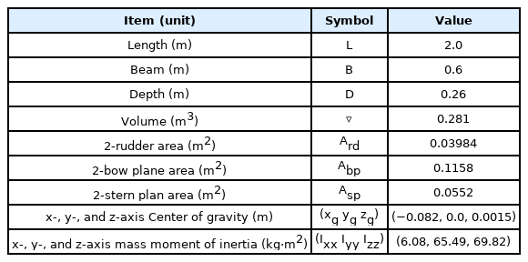
Principal parameters of the subject submerged body

2.3 Test Conditions

The conditions of the virtual captive model tests were configured, as presented in Table 2. Provided the CFD analysis is performed under the conditions in Table 2, all maneuvering coefficients can be obtained, excluding the coefficient related to thrust. All test conditions except a resistance test are applied with a design speed of 2.57 m/s (5 knots). Because there are two main thrusters attached in the rear part, yawing moment can be generated via steering and by thrust. Therefore, the submerged body may have a higher circular angular velocity than a submerged body that simply turns by steering, and the drift angle may also be larger because the circular angular velocity and drift angle are linked. Accordingly, a drift angle of approximately ±30° is considered when conducting a static drift test, as well as a dimensionless angular velocity of approximately 0.6. For self-propulsion, four auxiliary thrusters are attached to the hull, in addition to the main thrusters, and thrust can be freely generated in the vertical direction. Computation conditions were established considering an angle of attack of approximately ±90° because heave motions were realized by auxiliary thrusters. Hydrodynamic forces were computed using ANSYS FLUENT version 20.1, which is a commercial CFD analysis program. The analysis conditions adopted are presented in Table 3, and Fig. 3 illustrates the results obtained from mesh generation.

Table 2

Calculation matrix of virtual captive model tests

Table 3

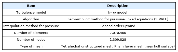
Analytic methods and conditions for CFD calculation

Fig. 3

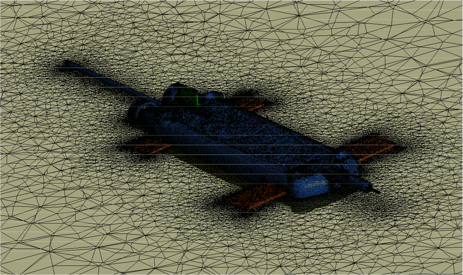
Mesh generation

The k– ω model is widely used to predict hydrodynamic forces applied on maneuvering ships (Quérard et al., 2008). The k– ω model for hydrodynamic derivatives is advantageous in terms of its CPU computation time. Because CFD calculations under several conditions are required in this study, the k– ω model was selected as the turbulence model. A 3D incompressible viscous flow was assumed, and a continuity equation and RANS equations were applied as governing equations (Jeon et al., 2016). The convection term was applied with the second-order upwind method, diffusion term was discretized using a second-order central differential method, and pressure and speed were linked by the semi-implicit method for pressure-linked equations (SIMPLE).

3. Analysis Results and Modeling

3.1 Static Test

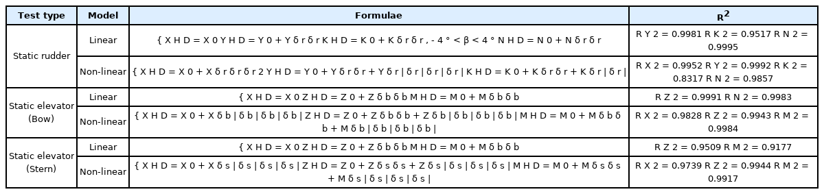
A static test estimates damping coefficients by calculating the damping force contributing to the speed of the hull and the rotation of a control plane, and it comprises resistance, static drift, static angle of attack, combined, static rudder, and static elevator tests. Details on the hydrodynamic force model of each test are presented in Table 4. The hydrodynamic force model was divided into two: a linear model in which the linearization of the force is possible because the size of perturbed state variables is small and a nonlinear model considering the nonlinearity of the force generated as motions become greater.

Table 4

Static hydrodynamic force model for hull motion variables

The results of the resistance test for estimating resistance per speed are presented in Fig. 4. When neutral buoyancy is assumed as the force proportional to the square of the advanced speed, approximately 9.8% of dead weight is assumed to be applied in the design speed. Here, dead weight refers to the product of the acceleration of gravity and the mass of the submerged body. Resistance is proportional to the square of the advanced speed, and the resistance applied on the hull can be linearized if the change in the speed is negligible, based on a design speed of 2.57 m/s (5 knots). Accordingly, Fig. 4 presents the results of the curve approximation of both linear and nonlinear models.

Fig. 4

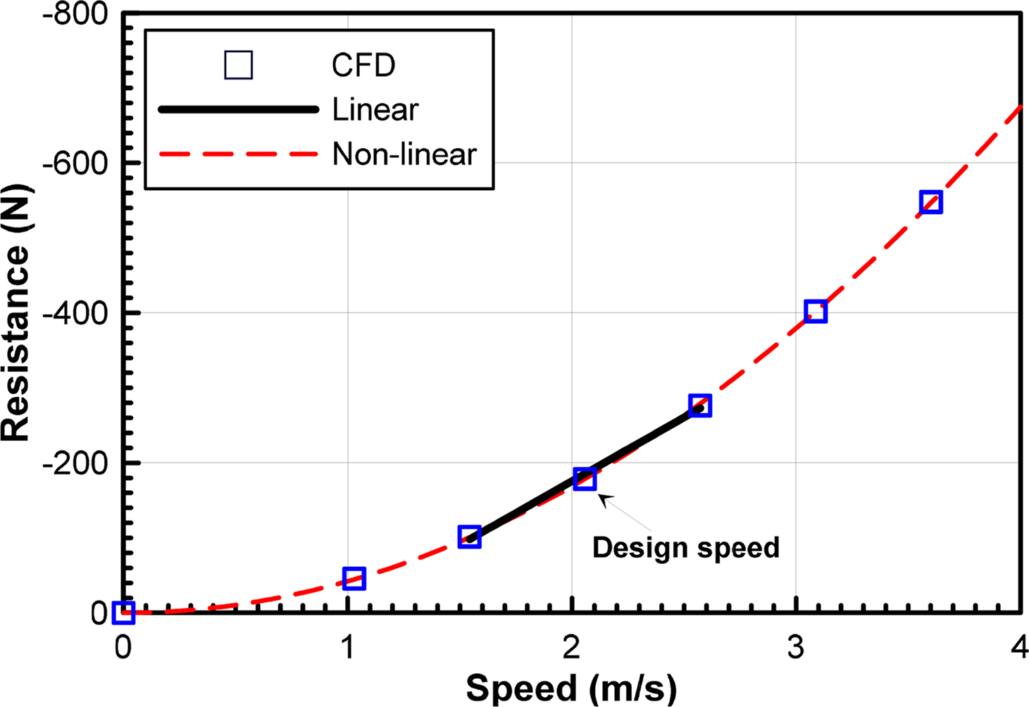
Result of resistance tests

A static drift test calculates the damping force applied when only the sway velocity is generated; the results obtained from calculating the force by adjusting the drift angle by ±30° are presented in Fig. 5. Nondimensionalization complies with the prime system 1 defined by the Society of Naval Architecture and Marine Engineering (SNAME) (Fossen, 2011). The hydrodynamic forces were modeled according to the tendency of forces. The nonlinear model presented in Table 3 was considered appropriate, and the coefficient of determination R² was approximately 1. In addition, linear coefficients were identified within the drift angle range of ±4°. As previously mentioned, hydrodynamic forces were calculated by adjusting the angle of attack by up to ±90°, considering a large angle of attack; the results obtained from the static angle of attack test are presented in Fig. 6. A stall occurs at approximately ±50° and ±40° of the surge and pitch, respectively, and the tendency of forces should be modeled using the same model as the static drift test. Nonlinear coefficients constituting the nonlinear model must be analyzed using simple curve approximation results because physical implication is ambiguous. In contrast, linear coefficients comprising the linear model have a distinct physical implication, such that the effectiveness of numerical analysis results can be determined by examining the correlation among linear coefficients when there are no experimental results, as in this study. Fig. 7 presents the points of damping force applications when the sway v and heave w velocities are generated based on the linear coefficients of stability Y_v, K_v, N_v, Z_w, and M_w, identified via the static drift and static angle of attack tests.

Fig. 5

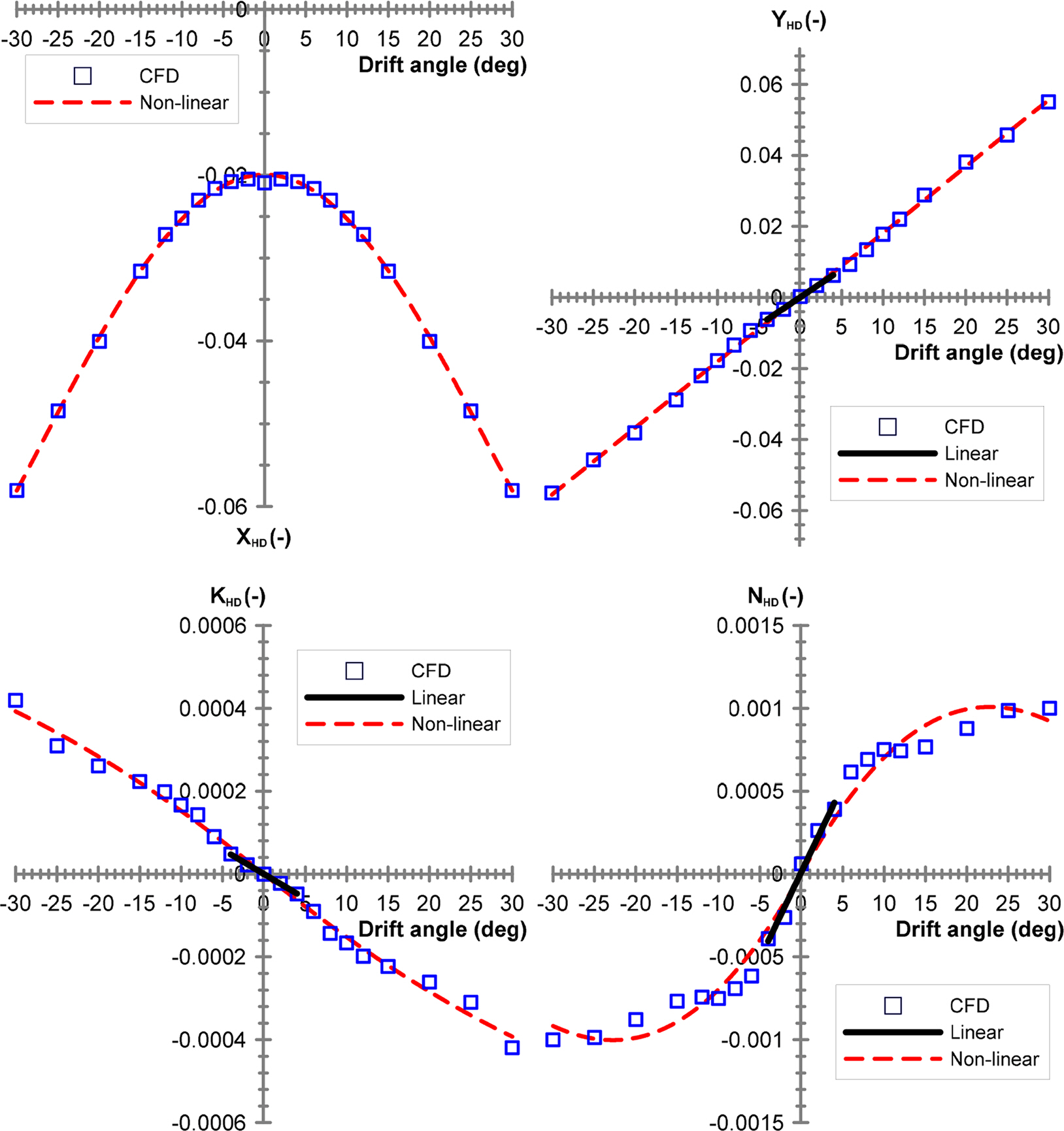
Results obtained from static drift tests

Fig. 6

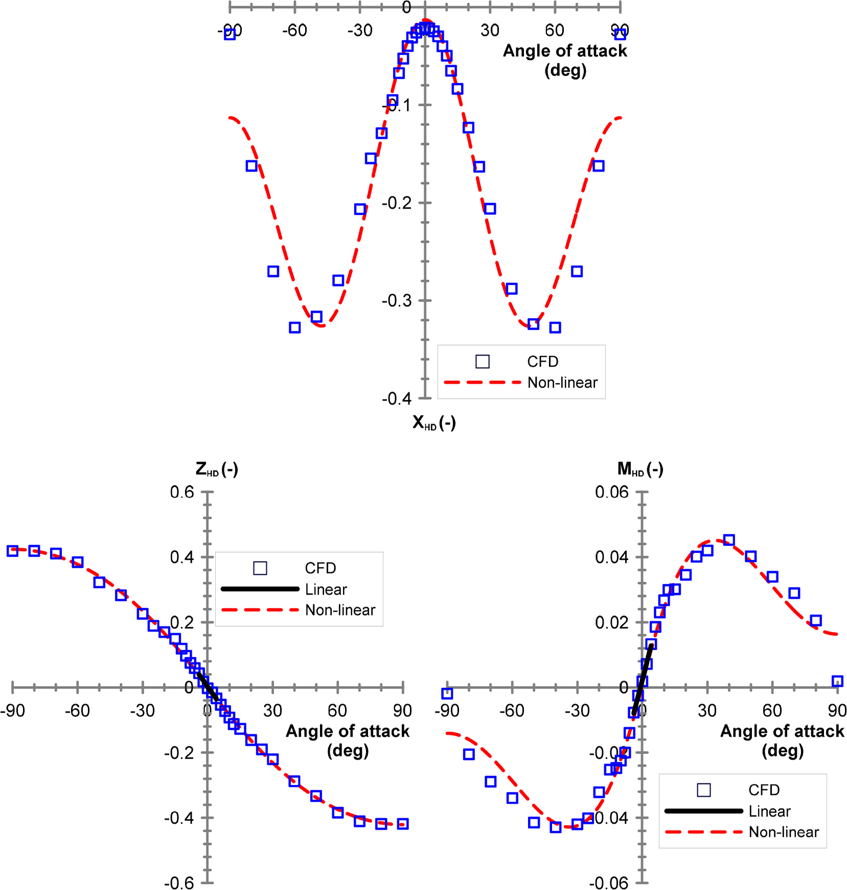
Results obtained from static angle of attack tests

Fig. 7

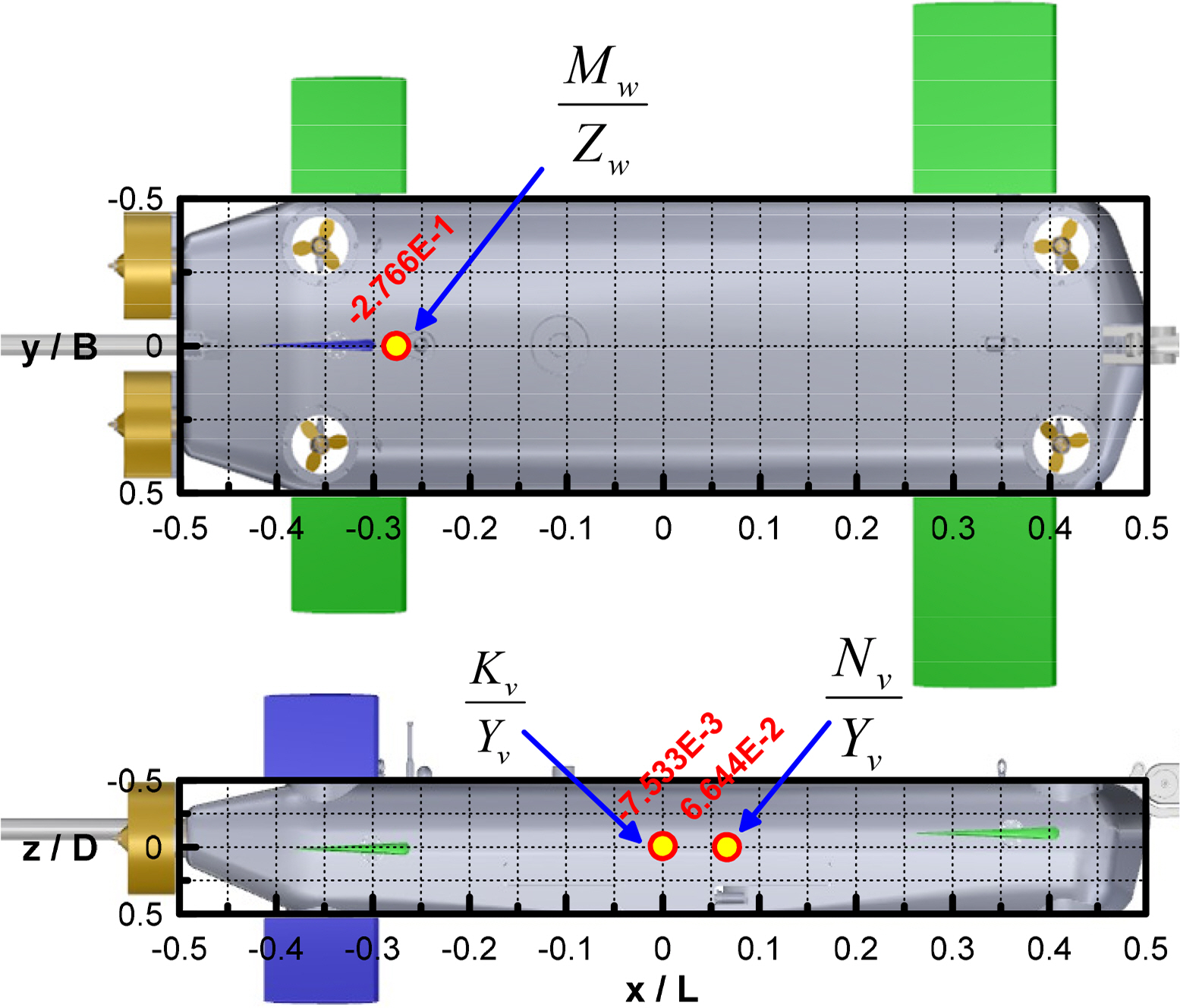
Moment levers due to heave (upper) and sway (lower) velocities

The side shape of the subject submerged body exhibits a tendency in which the rear part area is predominant owing to the large rudder attached in the rear part; thus, it is predicted to exhibit relatively better results in terms of horizontal stability. Therefore, N_v/Y_v, which is the application point of the damping force in the longitudinal direction due to the sway velocity, is positioned at approximately 0.066L in front of the origin. Considering that the N_v/Y_v of a general slender-type vehicle such as a ship is approximately 0.25L, the application point of the damping force moved backward considerably, toward the rear. Because the vertical shape is almost symmetrical, the application point K_v/Y_v of the damping force in the height direction is positioned slightly upward with respect to the geometrical origin; however, the size is negligible. In contrast, M_w/Z_w, which is the application point of the damping force in the longitudinal direction due to the heave velocity, is positioned approximately 0.277L toward the rear, with respect to the origin. A large bow plane exists in the head part, which implies that it is disadvantageous in terms of vertical stability, owing to the predominant head part.

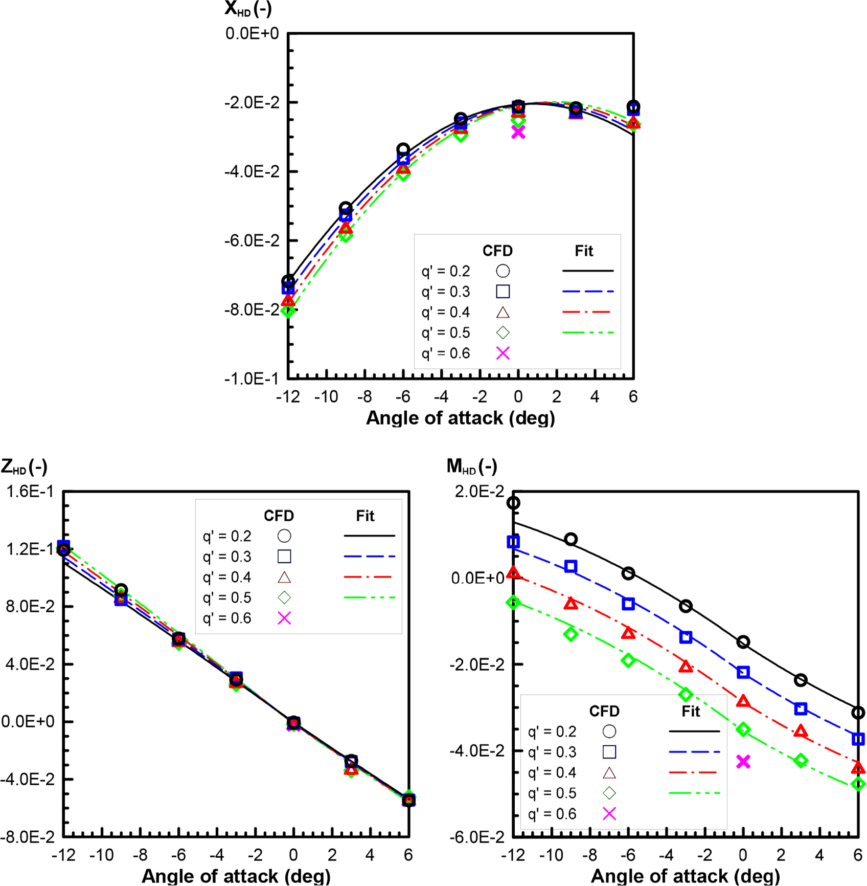
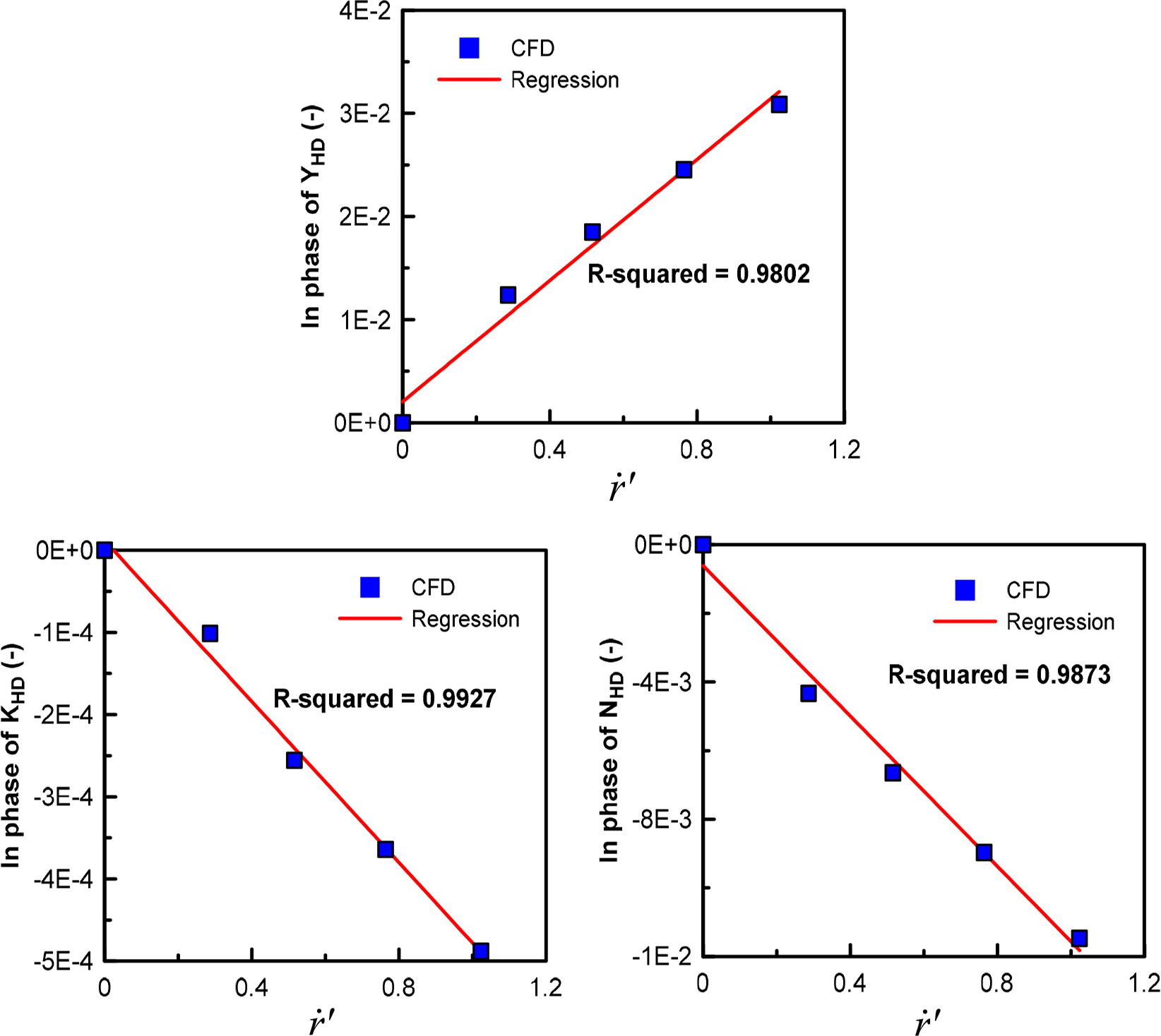
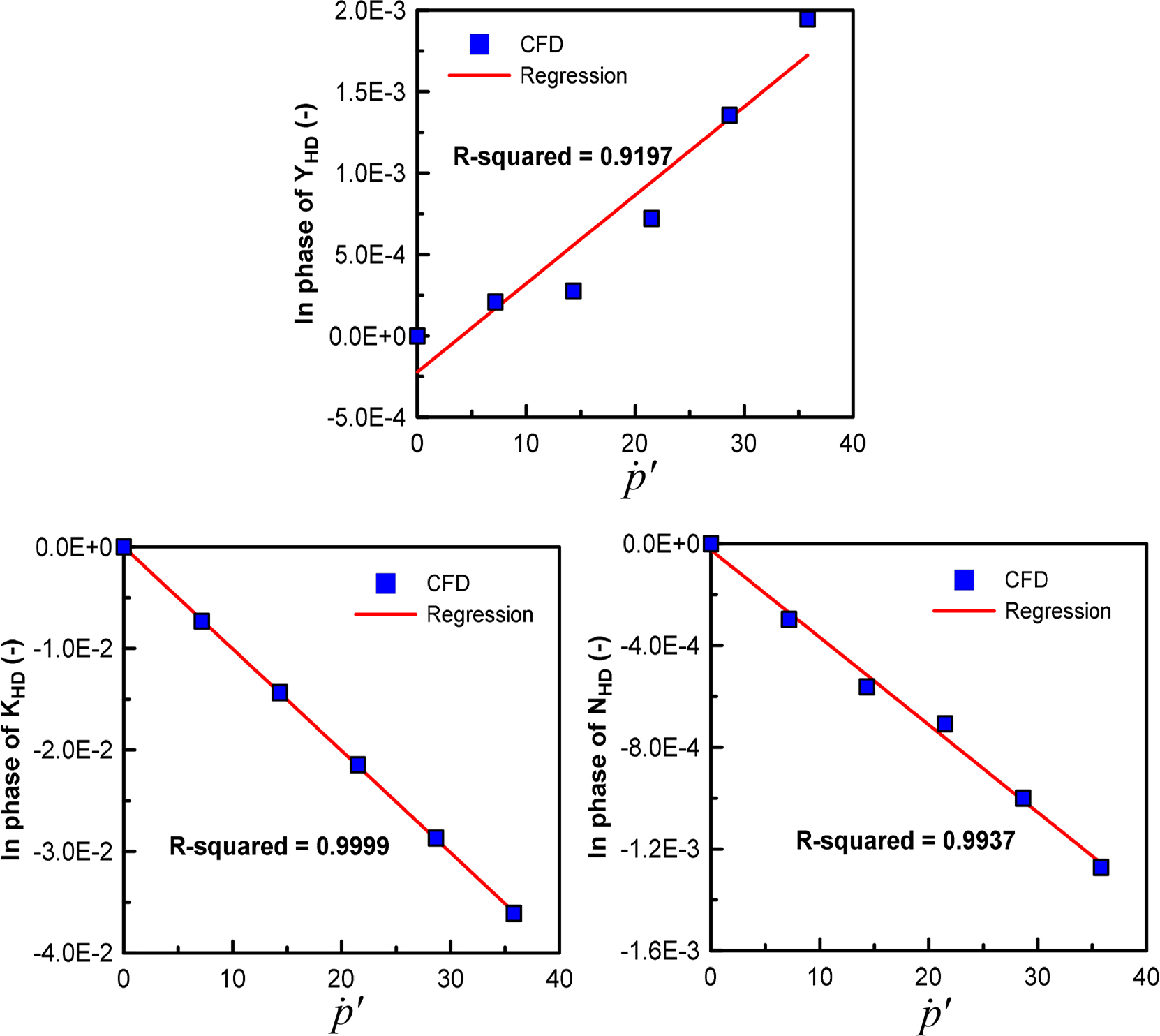
Figs. 8 and 9 present the results obtained from horizontal and vertical turning tests, which are conducted to determine the damping force and moment related to the yaw angular velocity r and pitch velocity q. The top area is more than two times greater than the side area of the hull, and the vertical hydrodynamic moment M_HD is substantially greater than the horizontal hydrodynamic moment Y_HD. In contrast, hydrodynamic forces Y_HD and Z_HD are the forces generated from the difference in the shapes of the head and rear parts during the rotational motions in which the asymmetry of the shapes of the head and rear parts significantly influence the horizontal hydrodynamic force Y_HD .

Fig. 8

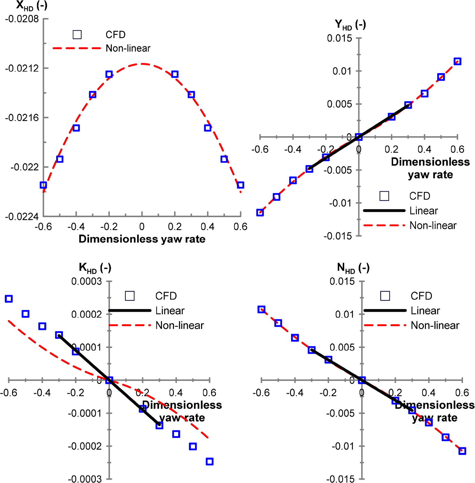
Results obtained from horizontal circular motion tests

Fig. 9

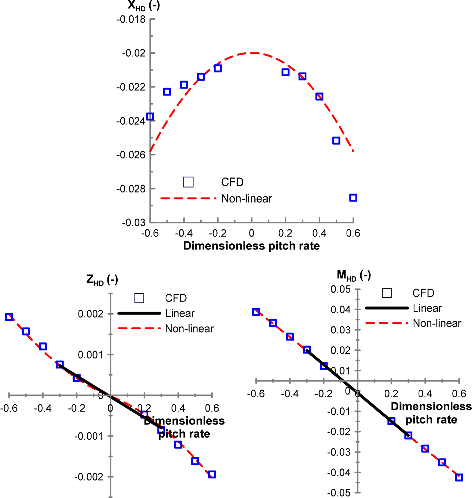
Results obtained from vertical circular motion tests

Fig. 10 presents the results of a roll rotating test, which measures the force generated by a certain roll rate p while a submerged body is advanced at speed U . Generally, a submerged body with a cylindrical shape frequently experiences a large rolling motion if a controller is not applied because the roll damping coefficient applied on the hull is relatively small. The subject submerged body in this study has a relatively flat hull top surface and a large elevator area, thus exhibiting a large roll damping moment. As shown in Fig. 10, which illustrates the roll damping moment K_HD for the roll rate p, the order is greater than that of the same angular motion moment N_HD . A large roll damping moment indicates that a roll is not large during circular motions in which favorable dynamic characteristics can be obtained from the motion control perspective. A simulation must be conducted to verify whether such a phenomenon actually occurs.

Fig. 10

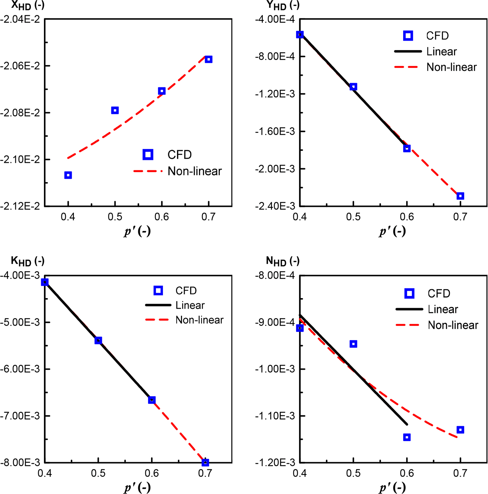
Results obtained from roll rotating tests

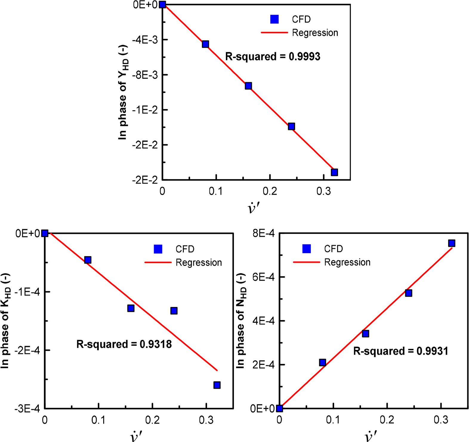
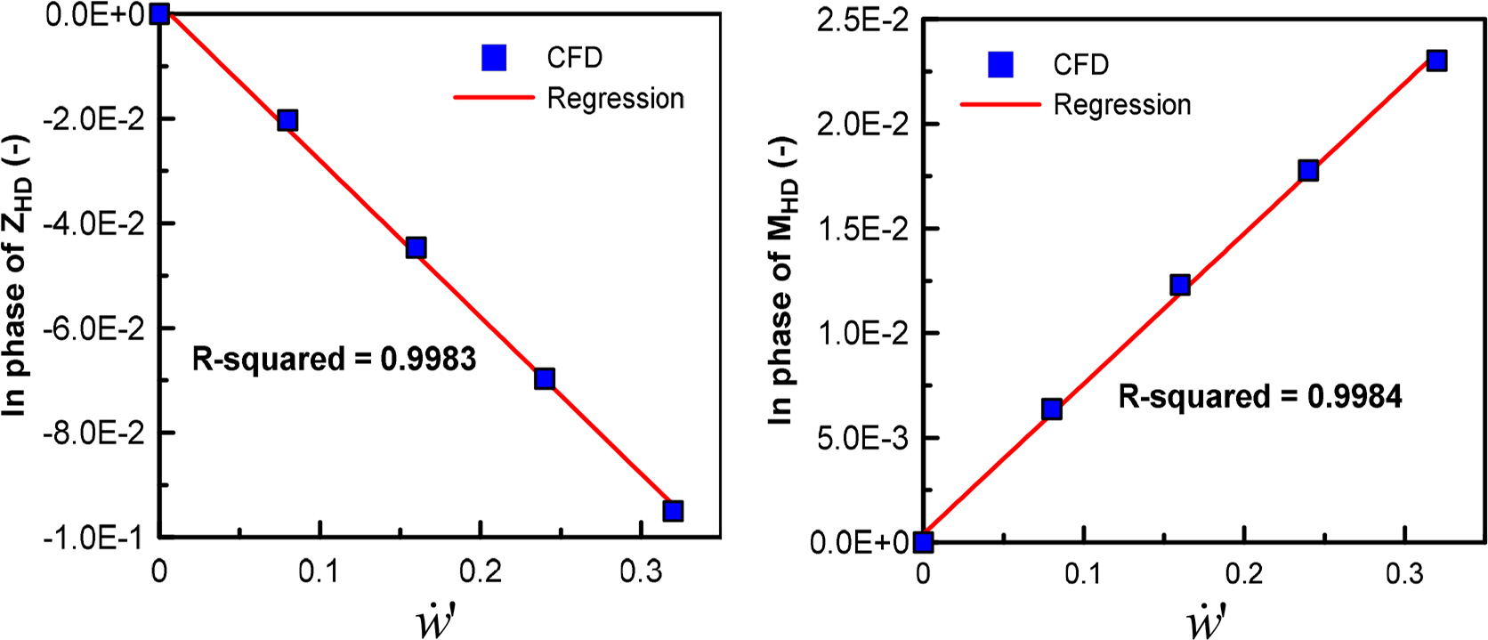
Figs. 11 and 12 present the results of the horizontal circular motion with the drift test and those of the vertical circular motion with the angle of attack test. The hydrodynamic forces measured in the static drift and horizontal turning tests are also measured when the horizontal circular motion with the drift test is performed; therefore, all hydrodynamic forces applied by and can be determined. Likewise, the hydrodynamic forces measured in the static angle of attack and vertical turning tests are also measured if the vertical circular motion is performed with drift test; therefore, all hydrodynamic forces applied by w and q can be determined.

Fig. 11

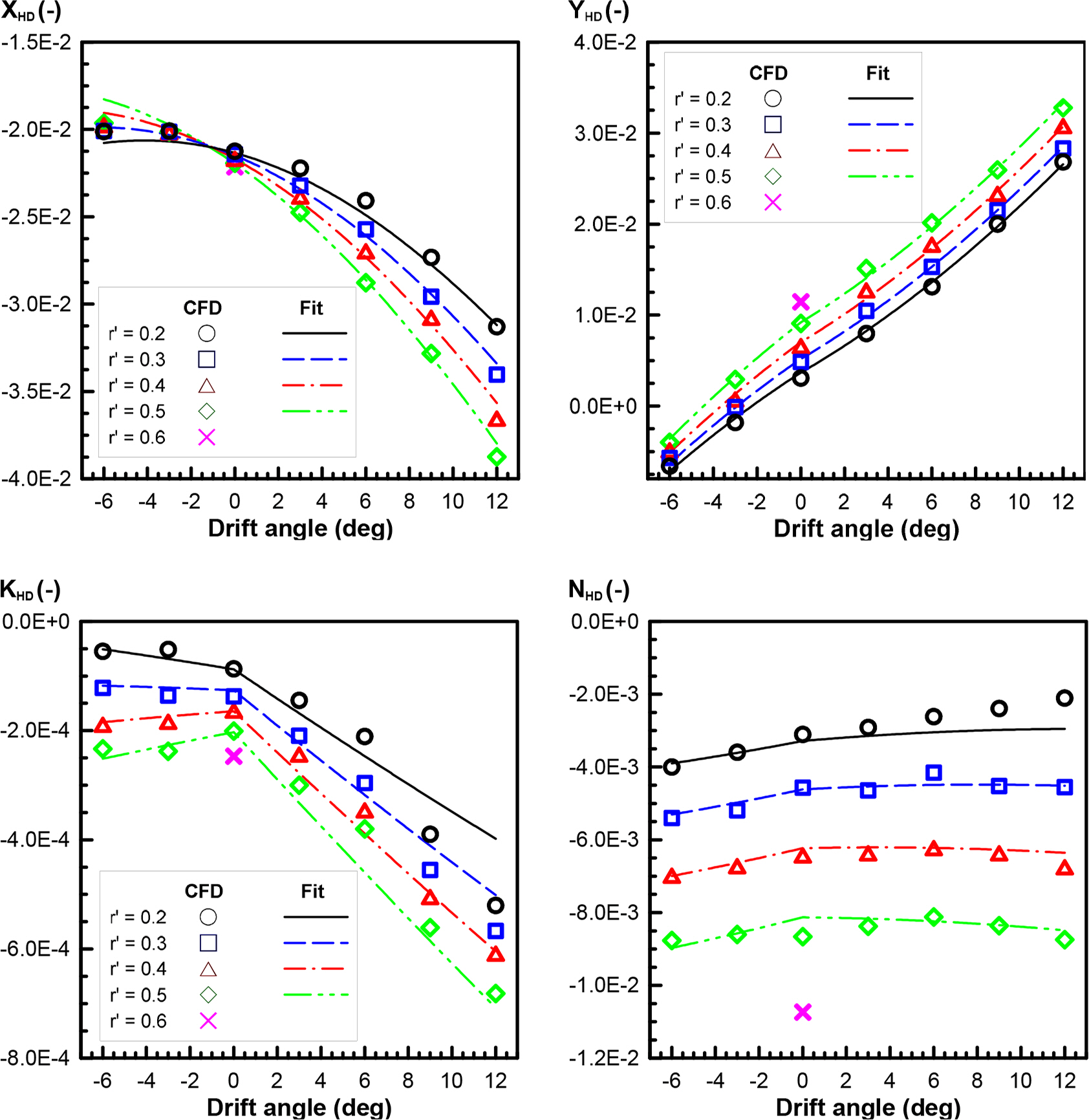
Results obtained from the horizontal circular motion with drift tests

Fig. 12

Results obtained from the vertical circular motion with the angle of attack tests

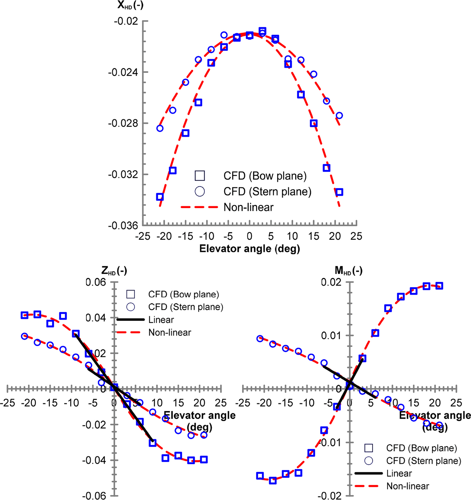
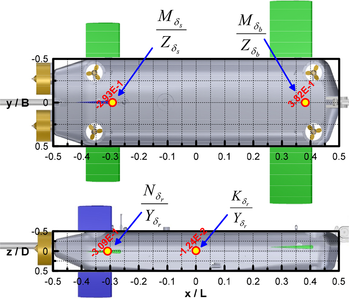
All the damping coefficients due to ship motions u, v, w, p, q, and r were estimated via the above tests. Table 5 presents the coefficient of determination of the hydrodynamic force model and corresponding models generated in the static rudder and static elevator tests. Figs. 13–14 present the results of the static rudder and static elevator tests, respectively. In general, the center of pressure of the hydrodynamic forces applied on a rudder is positioned at approximately 1/4 the point of a rudder chord. Similar to the static drift test, hydrodynamic forces and the rudder angle have a linear relationship in a region with a small rudder angle; hence, a linear coefficient can be determined to estimate the center of pressure of the rudder force. Fig. 15 presents the center of pressure on a rudder, which is estimated based on a linear coefficient when the rudder was rotated by a small angle. The center of pressure in the longitudinal direction N_{δ_r}/Y_{δ_r} when the rudder was rotated is positioned closer to 1/4 of a rudder chord. The center of pressure in the vertical direction K_{δ_r}/Y_{δ_r} is slightly more predominant in the top area from the side view of the hull; however, the size of K_{δ_r}/Y_{δ_r} is negligible because the vertical shape of the hull is almost symmetrical. The centers of pressure when the bow plane and stern elevator are turned, M_{δ_b}/Z_{δ_b} and M_{δ_s}/Z_{δ_s}, are also approximate to the 1/4 point of a rudder chord. Fig. 14 presents the results obtained from comparing the hydrodynamic forces when the bow plane was turned and when the stern elevator was turned. The area of a bow plane is approximately twice as large as the area of a stern elevator; hence, the linear control panel coefficient Z_{δ_b} provided in Table 6 is approximately twice as large as Z_{δ_s} . In contrast, moment coefficients M_{δ_b} and M_{δ_s} are associated with the distance to the pressure center of a control panel, and M_{δ_b} is at least two times greater than M_{δ_s} because the pressure center of a bow plane is far from the origin. Similarly, examining the physical relationship between linear coefficients appears to be an appropriate method for verifying the CFD analysis results when no experimental results are available.

Table 5

Static hydrodynamic force model for control plane angles

Fig. 13

Results obtained from static rudder tests

Fig. 14

Results obtained from static elevator tests

Fig. 15

Moment levers due to elevator (upper) and rudder (lower) deflections

Table 6

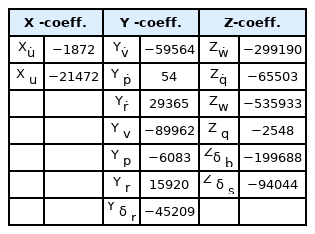
Dimensionless linear maneuvering mathematical model parameters (×10⁶)

3.2 Dynamic Test

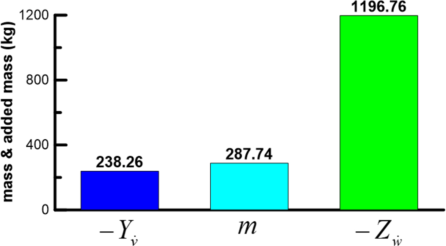
A dynamic test was performed to estimate the added mass force applied on the hull and the surrounding fluid when the hull accelerates. The added mass force exhibits a linear relationship with acceleration when a vessel or a submerged body has a very small accelerated motion. Figs. 16 and 17 present the results obtained from pure sway tests for estimating the added mass force with respect to sway acceleration v̇ and pure heave tests for estimating the added mass force with respect to heave acceleration ẇ, respectively. The added mass moment of inertia coefficients K_v̇ and N_v̇ for v̇ are typically negligible, as well as the added mass moment of inertia coefficient M_ẇ for ẇ; therefore, the sizes of Y_v̇ and Z_ẇ need to be examined. The results obtained from comparing the sizes of Y_v̇ and Z_ẇ with the mass of the submerged body are illustrated in Fig. 18. Y_v̇ of a general ship has proportion of its mass. Furthermore, Y_v̇ and Z_ẇ are identical in a submerged body with symmetrical horizontal and vertical planes. However, the subject submerged body in this study is applied with a relatively greater added mass force owing to its plate shape. Considering that the top surface area is at least twice as large as the side area and the top surface shape is a plate shape, rather than a streamlined shape, it is feasible for the size of Z_ẇ to be greater than that of Y_v̇ and its own mass.

Fig. 16

Results obtained from pure sway tests

Fig. 17

Results obtained from pure heave tests

Fig. 18

Comparison of mass and added mass

Figs. 19 –21 illustrate the results obtained from a dynamic test for angular acceleration. Figs. 19 and 20 present the results obtained from estimating added mass coefficients for yaw angular acceleration ṙ and pitch angular acceleration q̇. Similar to the difference in the sizes of Y_v̇ and Z_ẇ, the size of M_q̇ is greater than that of N_ṙ because the top surface shape is more predominant than that of the side shape. In general, the added mass moment of inertia is sufficiently small to be negligible compared to the mass moment of inertia (I_xx) in a submerged body with a streamlined shape when a roll angular acceleration ṗ is generated. However, the subject submerged body has a relatively plate-like shape, and the slenderness ratio (L/B) is relatively small. Moreover, a large hydrodynamic moment is generated by a roll angular acceleration because the areas of bow and stern elevators are large. Consequently, the yaw induced mass moment of inertia K_ṗ is relatively larger than that of a general slender-type submerged body, as illustrated in Fig. 21.

Fig. 19

Results obtained from pure yaw tests

Fig. 20

Results obtained from pure pitch tests

Fig. 21

Results obtained from pure roll tests

3.3 Dynamics Model

The six degrees-of-freedom equations of motion based on Newton’s second law of motion can be expressed as in Eq. (1).

(1) {m[u˙-vr+wq-xg(q2+r2)+zg(pr+q˙)]=Xm[v˙-wp+ur+zg(qr+p˙)+xg(qp+r˙)]=Ym[w˙-uq+vp-zg(r2+p2)+xg(rp+q˙)]=ZIxp˙+(Iz-Iy)qr-m[zg(v˙-wp+ur)]=KIyq˙+(Ix-Iz)rp+m[zg(u˙-vr+wq)-xg(w˙-wq+vp)]=MIzr˙+(Iy-Ix)pq+m[xg(v˙-wp+ur)]=N

External forces on the right side of Eq. (1) can be divided into hydrodynamic force, gravitational force, buoyant force, control force, and thrust. Hydrodynamic forces were modeled as expressed in Eqs. (2) and (3) by distinguishing linear models for designing the controller and stability analysis and nonlinear models for predicting maneuverability based on the coefficients identified via the static and dynamic tests.

(2) {XHD=Xu˙u˙+XuuYHD=Yv˙v˙+Yp˙p˙+Yr˙r˙+Yvv+Ypp+YrrZHD=Zw˙w˙+Zq˙q˙+Zww+ZqqKHD=Kv˙v˙+Kp˙p˙+Kr˙r˙+Kvv+Kpp+KrrMHD=Mw˙w˙+Mq˙q˙+Mww+MqqNHD=Nv˙v˙+Np˙p˙+Nr˙r˙+Nvv+Npp+Nrr

(3) {XHD=Xu˙u˙+Xu|u|u|u|+Xvvv2+Xvvvvv4+Xwww2+Xwwwww4+Xppp2+Xqqq2+Xrrr2+Xvrvr+XwqwqYHD=Yv˙v˙+Yp˙p˙+Yr˙r˙+Yvv+Ypp+Yrr+Yv|v|v|v|+Yp|p|p|p|+Yr|r|r|r|+Yv|r|v|r|+Y|v|r|v|rZHD=Zw˙w˙+Zq˙q˙+Z*+Zww+Zqq+Zw|w|w|w|+Zq|q|q|q|+Zw|q|w|q|+Z|w|q|w|q{KHD=Kv˙v˙+Kp˙p˙+Kr˙r˙+Kvv+Kpp+Krr+Kv|v|v|v|+Kp|p|p|p|+Kr|r|r|r|+Kv|r|v|r|+K|v|r|v|rMHD=Mw˙w˙+Mq˙q˙+Z*+Mww+Mqq+Mw|w|w|w|+Mq|q|q|q|+Mw|q|w|q|+M|w|q|w|qNHD=Nv˙v˙+Np˙p+Nr˙r˙+Nvv+Npp+Nrr+Nv|v|v|v|+Np|p|p|p|+Nr|r|r|r|+Nv|r|v|r|+N|v|r|v|r

(4) {XC=0YC=YδrδrZC=Zδbδb+ZδsδsKC=KδrδrMC=Mδbδb+MδsδsNC=Nδrδr

(5) {XC=Xδrδrδr2YC=Yδrδr+Yδr|δr|δr|δr|ZC=Zδbδb+Zδsδs+Zδb|δb|δb|δb|+Zδs|δs|δs|δs|KC=Kδrδr+Kδr|δr|δr|δr|MC=Mδbδb+Mδsδs+Mδb|δb|δb|δb|+Mδs|δs|δs|δs|NC=Nδrδr+Nδr|δr|δr|δr|

Unlike other external forces contributing to the surface force, gravitational force and buoyancy are body forces that contribute to the volume, which do not require a modeling process as hydrodynamic forces, and can be perfectly expressed physically. Therefore, the expressions for gravitational force and buoyancy are omitted in this study because they can be referenced in the study by Fossen (2011). A control force is a fluid force applied on the control panel and the hull when the control panel rotates. Eqs. (4) and (5) represent the control force of linear and nonlinear models, respectively. The parameters expressed in Eqs. (2)–(5) are presented in Tables 6 and 7 by distinguishing between a linear and nonlinear model.

Table 7

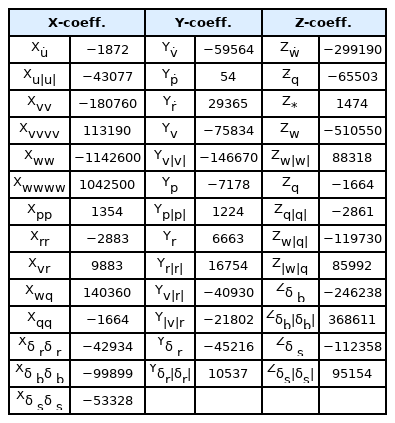
Dimensionless non-linear maneuvering mathematical model parameters (×10⁶)

Because the system has six thrusters attached, the subjectsubmerged body can create thrust in all directions, except for the sway direction. Thrust force with six degrees of freedom generated by each thruster can be defined as expressed in Eq. (6), based on Fig. 22.

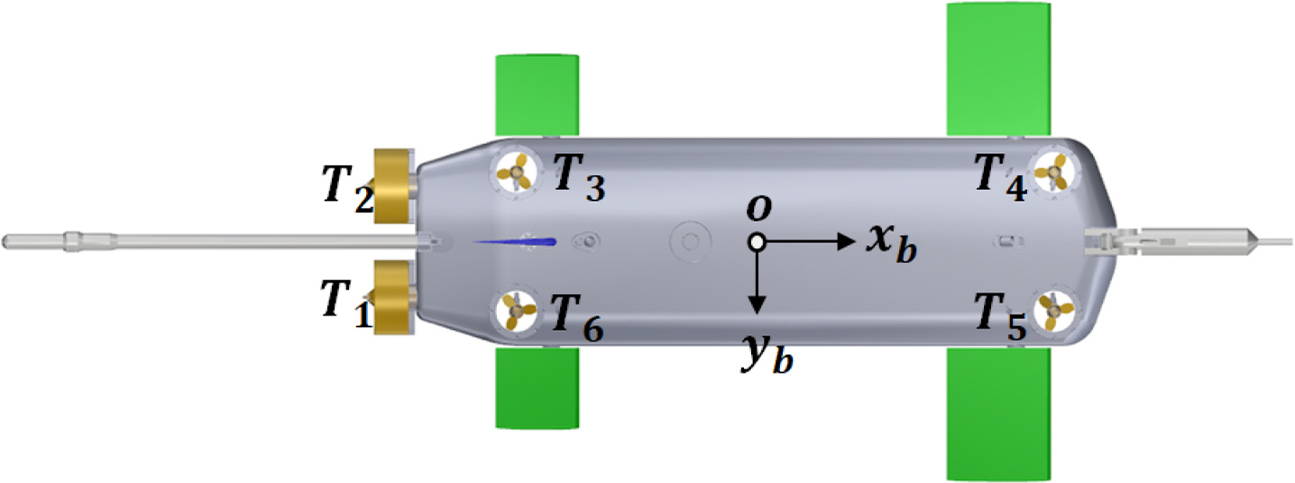
(6) {XT=T1+T2YT=0ZT=T3+T4+T5+T6KT=yT3T3+yT4T4+yT5T5+yT6T6MT=zT1T1+zT2T2-(xT3T3+xT4T4+xT5T5+xT6T6)NT=-(yT1T1+yT2T2)

Fig. 22

Sequence of thruster

x_{T_i}, y_{T_i}, and z_{T_i} in Eq. (6) represent the distance from the origin of the i-th thruster to the x-, y-, z-axes, respectively. The thrust specified in the specifications of each thrust manufacturer was adopted as the thrust defined by T_1–6.

4. Dynamics Simulation

4.1 Stability Analysis

A stability analysis was conducted to evaluate the stability relative to the ship’s course and depth while the control panel is fixed (δ_r = δ_b = δ_s = 0). The sizes of the perturbation state variables v, w, q, and r were not significant when the control panel was fixed and the linearization of the equations of motion in Eq. (1) was possible; hence, the linear stability coefficients in Table 6 were adopted. Horizontal and vertical stability can be evaluated based on the stability margin, under the assumption that surge velocity u has no influence on sway, yaw, heave, or pitch. Horizontal and vertical stability margins can be defined by adopting Eqs. (7) and (8), respectively, at infinite speed.

(7) Gh=1-Nv(Yr-m)Yv(Nr-mxg)

(8) Gv=1-Mv(Zq+m)Zw(Mq-mxg)

Because m and x_g in Eqs. (7)–(8) are design variables, the stability margin results in Fig. 23 can be deduced for x_g under the assumption that neutral buoyancy is applied. As mentioned in Section 3, the rear is more critical with regard to the side shape of the submerged body, where it was assumed to be more important than the vertical plane in terms of stability. The analysis results indicated that G_h is greater than G_v when the center of gravity is closer to zero.

Fig. 23

Results obtained from pure roll tests

4.2 Maneuverability Analysis

Unlike a stability analysis in which the control panel is fixed, the control panel can be adjusted to the maximum angle when analyzing maneuverability, such as in turning and veering, which creates large motions such as drifting or yaw rate. Therefore, the hydrodynamic and control forces defined in Eqs. (3) and (5) are required. A turning simulation was performed by altering the rudder angle by ±5°, ±10°, and ±15° under an initial speed of 2.57 m/s, and the obtained results are illustrated in Figs. 24 and 25. The simulation results indicate that the tactical diameter is approximately 7.42 m when the rudder angle is 15°. The hull length of the subject submerged body is 2 m, and the entire length is approximately 3.7 m, including a towing poll; hence, adequate turning performance is realized owing to the small side surface area and large rudder area. Through simulations, it was verified that the roll convergence was approximately 1° during turning owing to a relatively large roll damping moment which was due to the large elevator and top surface areas of the hull, as observed in the pure roll tests mentioned in Section 3. The result of a meander test, which evaluates vertical stability in the maneuverability test of the submerged body, is illustrated in Fig. 26. The meander test investigates the stability of motions in the vertical plane direction over time, after the disturbance of a certain size is applied in the vertical plane direction (Jeon et al., 2020). After generating disturbance for a specific time in the vertical plane direction by turning the bow plane and stern elevator, the test examines whether the depth is maintained over time when the elevator is turned again at an angle of 0°. Unlike horizontal plane motions, the vertical plane motions have a restoring moment, which is expressed as the sum of gravitational force and buoyancy, and thus converges to a specific value without diverging to a pitch angle. When the subject submerged body is assumed to be under neutral buoyancy, the pitch angle converges to zero, and the depth is maintained after the rudder angle is maintained at 0° after 30 s, as illustrated Fig. 26. Vertical stability can be examined again via a meander simulation, based on the results presented in Fig. 23. The motions in a large angle of attack were simulated by generating thrust and thrust moment in heave and pitch directions, while increasing the thrust of auxiliary thrusters T₃, T₄, T₅, and T₆ attached on the hull presented in Fig. 22 to 49 N, 98 N, and 147 N; the obtained results are presented in Fig. 27.

Fig. 24

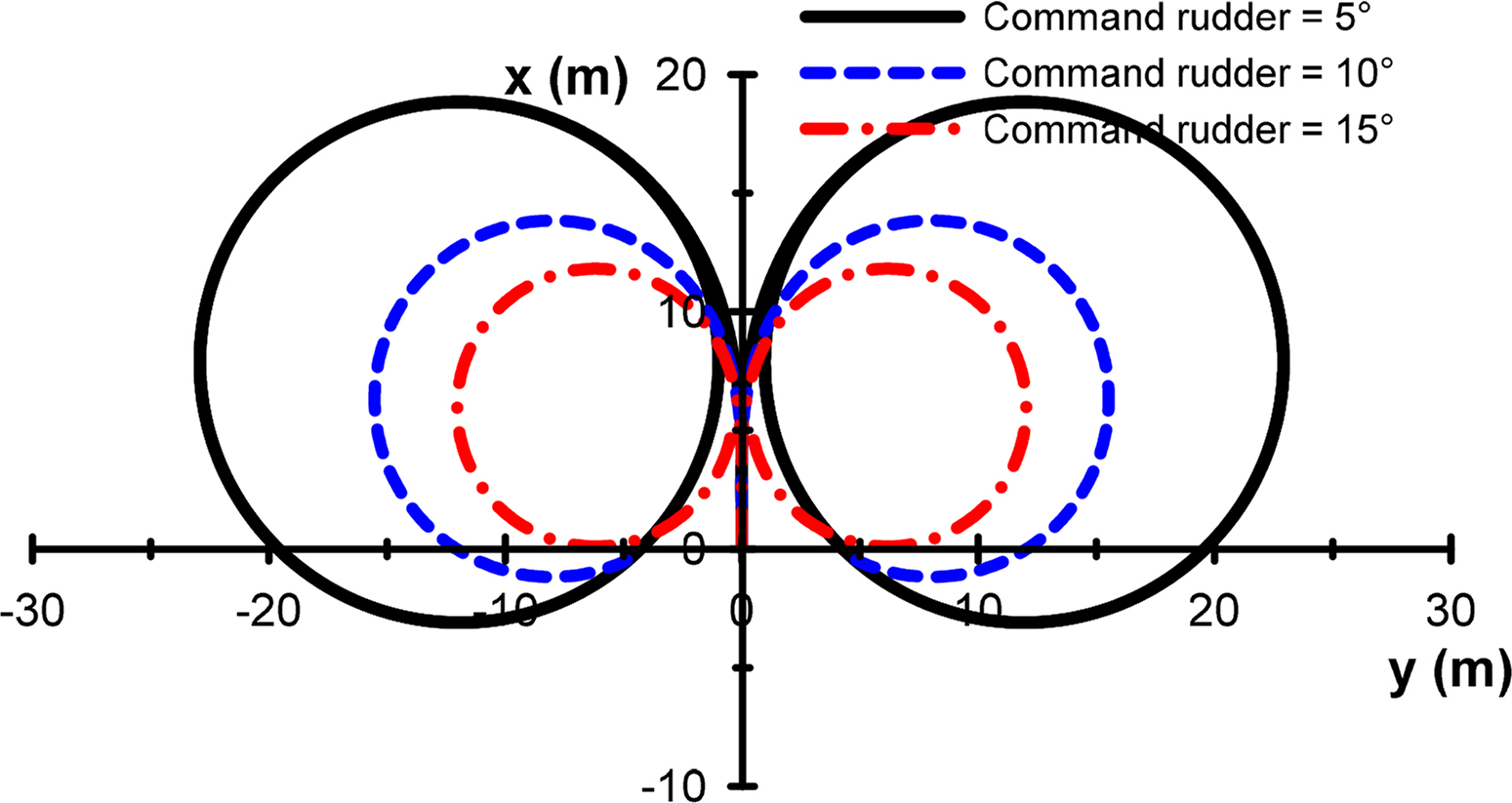
Trajectories of turning tests

Fig. 25

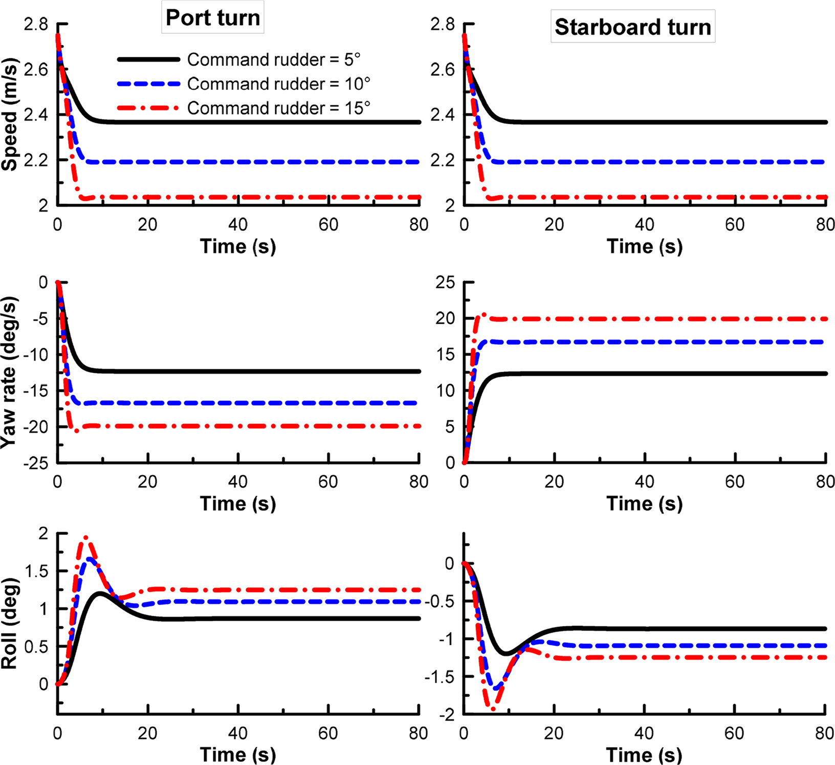
Motion variables of turning tests

Fig. 26

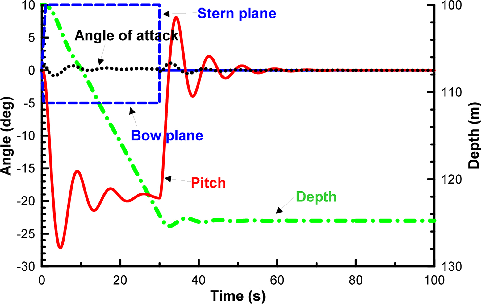
Meander test

Fig. 27

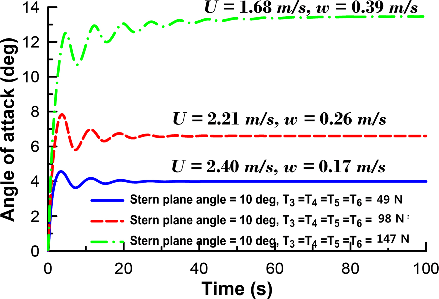
Large angle of attack test

5. Concluding Remarks

Maneuvering coefficients for a hydrodynamic model were estimated by performing virtual captive model tests based on CFD for a submerged body that can exhibit large angles of attack and receives various control inputs. The conditions for the virtual captive model tests based on CFD were established by considering that the subject submerged body has a large control panel area and exhibits a large angle of attack motion. A practical inference method was established to verify the results using the linear coefficients of the submerged body because no experimental results were available. Maneuvering coefficients were identified by distinguishing a linear model from a nonlinear model, based on the results of the static test. In general, the determination coefficients of the linear model were closer to 1 than those of nonlinear coefficients in the CFD analysis results, which implied that errors occurred in a mathematical model of hydrodynamic forces as drift angle and angle of attack increased. The accuracy of the mathematical model improved as the order of hydrodynamic derivatives increased; however, the structural stability of the mathematical model of hydrodynamic forces reduced accordingly. The mathematical model was appropriately established because the determination coefficients were generally 0.95 or higher. Because linear coefficients have significant physical implications, the application point of a damping force was verified when a small perturbed motion was generated. Moreover, the application point of the damping force was realistic when the motion of the hull and rotation of the control panel occurred. Dynamic characteristics of the submerged body were evaluated by establishing a mathematical model with six degrees of freedom for thrust generated by six thrusters and hydrodynamic forces applied on the hull by a large angle of attack motion and the rotation of the control panel. Excellent turning characteristics were obtained because the rudder area was larger than the side surface area of the hull, and the stability of the vessel’s course was secured. Arbitrary thrust was applied to the auxiliary thrusters attached to the hull, and the large angle of attack motion in the vertical direction was simulated by changing the elevator; however, the effect of the design variables, including the weight of the submerged body and its center of gravity, were greater. The hydrodynamic model will be further improved by tuning various coefficients and comparing the results of an actual experiment with the results of a CFD analysis.

Nomenclature

O – xyz

Earth-fixed coordinate

o – x_by_bz_b

Body-fixed coordinate

Vehicle speed (m/s)

Drift angle (deg)

Angle of attack (deg)

Surge (axial) velocity (m/s)

Sway (lateral) velocity (m/s)

Heave (vertical) velocity (m/s)

Roll rate (deg/s)

Pitch rate (deg/s)

Yaw rate (deg/s)

δ_r

Rudder angle (deg)

δ_b

Bow plane angle (deg)

δ_s

Stern plane angle (deg)

X_u̇

Derivative of X_HD with respect to u̇

X_u

Derivative of X_HD with respect to u

X_u_|_u_|

Derivative of X_HD with respect to u|u|

X_{δ_b|δ_b|}

Derivative of X_C with respect to δ_b|δ_b|

X_{δ_s|δ_s|}

Derivative of X_C with respect to δ_s|δ_s|

X_{δ_r|δ_r|}

Derivative of X_C with respect to δ_r|δ_r|

Y_v̇

Derivative of Y_HD with respect to v̇

Y_ṗ

Derivative of Y_HD with respect to ṗ

Y_ṙ

Derivative of Y_HD with respect to ṙ

Y_v

Derivative of Y_HD with respect to v

Y_p

Derivative of Y_HD with respect to p

Y_r

Derivative of Y_HD with respect to r

Y_{δ_r}

Derivative of Y_C with respect to δ_r

Z_ẇ

Derivative of Z_HD with respect to ẇ

Z_q̇

Derivative of Z_HD with respect to q̇

Z_w

Derivative of Z_HD with respect to w

Z_q

Derivative of Z_HD with respect to q

Z_{δ_b}

Derivative of Z_C with respect to δ_b

Z_{δ_s}

Derivative of Z_C with respect to δ_s

K_v̇

Derivative of K_HD with respect to v̇

K_ṗ

Derivative of K_HD with respect to ṗ

K_ṙ

Derivative of K_HD with respect to ṙ

K_v

Derivative of K_HD with respect to v

K_p

Derivative of K_HD with respect to p

K_r

Derivative of K_HD with respect to r

K_{δ_r}

Derivative of K_C with respect to δ_r

M_ẇ

Derivative of M_HD with respect to ẇ

M_q̇

Derivative of M_HD with respect to q̇

M_w

Derivative of M_HD with respect to w

M_q

Derivative of M_HD with respect to q

M_{δ_b}

Derivative of M_C with respect to δ_b

M_{δ_s}

Derivative of M_C with respect to δ_s

N_v̇

Derivative of N_HD with respect to v̇

N_ṗ

Derivative of N_HD with respect to ṗ

N_ṙ

Derivative of N_HD with respect to ṙ

N_v

Derivative of N_HD with respect to v

N_p

Derivative of N_HD with respect to p

N_r

Derivative of N_HD with respect to r

N_{δ_r}

Derivative of N_C with respect to δ_r

Notes

This research was financially supported by the Institute of Civil Military Technology Cooperation, funded by the Defense Acquisition Program Administration and Korean government Ministry of Trade, Industry, and Energy.

References

Bae J.-Y, Sohn K.-H. 2009;A Study on Manoeuvring Motion Characteristics of Manta-type Unmanned Undersea Vehicle. Journal of the Society of Naval Architects of Korea 46(2):114–126. https://doi.org/10.3744/snak.2009.46.2.114 .

Cho YJ, Seok W, Cheon K.-H, Rhee SH. 2020;Maneuvering Simulation of an X-plane Submarine Using Computational Fluid Dynamics. International Journal of Naval Architecture and Ocan Engineering 12:843–855. https://doi.org/10.1016/j.ijnaoe.2020.10.001 .

Fossen TI. 2011. Handbook of Marine Craft Hydrodynamics and Motion Control New Jersey, USA: John Wiley & Sons.

Jeon M, Lee D, Yoon HK, Koo B. 2016;Modeling and Tracking Simulation of ROV for Bottom Inspection of a Ship using Component Drag Model. Journal of Ocean Engineering and Technology 30(5):374–380. https://doi.org/10.5574/ksoe.2016.30.5.374 .

Jeon M, Nguyen TT, Yoon HK, Cho HJ. 2020;A Study on Verification of the Dynamic Modeling for a Submerged Body Based on Numerical Simulation. International Journal of Engineering and Technology Innovation 10(2):107–120. https://doi.org/10.46604/ijeti.2020.4350 .

Jeon M, Yoon HK, Hwang J, Cho HJ. 2017;Study on Maneuvering Characteristics of Submerged Body by Changing Its Design Parameters. Journal of Ocean Engineering and Technology 31(2):155–163. https://doi.org/10.5574/ksoe.2017.31.2.155 .

Jung J.-W, Jeong JH, Kim IG, Lee S.-K. 2014;Experimental Study on Hydrodynamic Coefficients of Autonomous Underwater Glider Using Vertical Planar Motion Mechanism Test. Journal of Ocean Engineering and Technology 28(2):119–125. https://doi.org/10.5574/ksoe.2014.28.2.119 .

Kim Y.-G, Yun K.-H, Kim S.-Y, Kim D.-J. 2012;Captive Model Test of Submerged Body Using CPMC. Journal of the Society of Naval Architects of Korea 49(4):296–303. https://doi.org/10.3744/snak.2012.49.4.296 .

Nguyen TT, Yoon HK, Park Y, Park C. 2018;Estimation of Hydrodynamic Derivatives of Full-Scale Submarine using RANS Solver. Journal of Ocean Engineering and Technology 32(5):386–392. https://doi.org/10.26748/ksoe.2018.6.32.5.386 .

Park J.-Y, Kim N, Rhee K.-P, Yoon HK, Kim C, Jung C, Lee S. 2015;Study on Coning Motion Test for Submerged Body. Journal of Ocean Engineering and Technology 29(6):436–444. https://doi.org/10.5574/ksoe.2015.29.6.436 .

Quérard A, Temarel P, Turnock S. 2008. Influence of Viscous Effects on the Hydrodynamics of Ship-Like Section Undergoing Symmetric and Anti-Symmetric Motions Using RANS. In : Proceedings of the 27th International Conference on Offshore Mechanics and Arctic Engineering. Estoril, Portugal. p. 683–692. https://doi.org/10.1115/OMAE2008-57330 .

Yeo DJ, Yoon HK, Kim YG, Lee CM. 2006;Sensitivity Analysis on the Stability of a Submarine Concerning its Design Parameters. Journal of the Society of Naval Architects of Korea 12:843–855. https://doi.org/10.1016/j.ijnaoe.2020.10.001 .

Takashina J. 1986;Ship Maneuvering Motion due to Tugboats and Its Mathematical Model. Journal of the Society of Naval Architects of Japan 160:93–102. https://doi.org/10.2534/jjasnaoe1968.1986.160_93 .

Yoon HK, Kim SY. 2005;A Study on the Model Test Scheme for Establishing the Mathematical Model of Hydrodynamic Force and Moment Acting on a Slowly Moving Ship. Journal of the Society of Naval Architects of Korea 42(2):98–104. https://doi.org/10.3744/SNAK.2005.42.2.098 .

Article information Continued

This is an open access article distributed under the terms of the creative commons attribution non-commercial license (http://creativecommons.org/licenses/by-nc/4.0) which permits unrestricted non-commercial use, distribution, and reproduction in any medium, provided the original work is properly cited.

Item (unit)	Symbol	Value
Length (m)	L	2.0
Beam (m)	B	0.6
Depth (m)	D	0.26
Volume (m³)	▿	0.281
2-rudder area (m²)	A_rd	0.03984
2-bow plane area (m²)	A_bp	0.1158
2-stern plan area (m²)	A_sp	0.0552
x-, y-, and z-axis Center of gravity (m)	(x_g y_g z_g)	(−0.082, 0.0, 0.0015)
x-, y-, and z-axis mass moment of inertia (kg·m²)	(I_xx I_yy I_zz)	(6.08, 65.49, 69.82)

Test type	Motion variables
Resistance test	U = 1.03, 1.54, 2.06, 2.57, 3.09, 3.60 m/s (2.0, 3.0, 4.0, 5.0, 6.0, 7.0 knot)
Static drift test	β = ±2°, ±4°, ±6°, ±8°, ±10°, ±12°, ±15°, ±20°, ±25°, ±30°
Static angle of attack test	α = ±2°, ±4°, ±6°, ±8°, ±10°, ±12°, ±15°, ±20°, ±25°, ±30°, ±40°, ±50°, ±60°, ±70°, ±80°, ±90°
Horizontal circular motion test	r′ = ±0.2, ±0.3, ±0.4, ±0.5, ±0.6
Vertical circular motion test	q′= ±0.2, ±0.3, ±0.4, ±0.5, ±0.6
Horizontal circular motion with drift test	β = ±2°, ±4°, ±6°, +8°, +10°, +12° r′ = 0.2, 0.3, 0.4, 0.5
Vertical circular motion with angle of attack test	α = ±2°, ±4°, ±6°, −8°, −10°, −12° q′ = 0.2, 0.3, 0.4, 0.5
Static rudder test	δ_r = ±3°, ±6°, ±9°, ±12°, ±15°, ±18°, ±21°
Static elevator test (bow plane)	δ_b = ±3°, ±6°, ±9°, ±12°, ±15°, ±18°, ±21°
Static elevator test (stern plane)	δ_s = ±3°, ±6°, ±9°, ±12°, ±15°, ±18°, ±21°
Roll rotating test	p′ = 0.4, 0.5, 0.6, 0.7
Pure sway test	v̇′ = 0.08, 0.16, 0.24, 0.32
Pure yaw test	ṙ′ = 0.29, 0.52, 0.76, 1.02
Pure heave test	ẇ′ = 0.08, 0.16, 0.24, 0.32
Pure pitch test	q̇′ = 0.29, 0.52, 0.76, 1.02
Pure roll test	ṗ′ = 7.2, 14.3, 21.5, 28.6, 35.8

Item	Description
Turbulence model	k– ω model
Algorithm	Semi-implicit method for pressure-linked equations (SIMPLE)
Interpolation method for pressure	Second order upwind
Number of elements	7,070,460
Number of nodes	1,309,828
Type of mesh	Tetrahedral unstructured mesh, Prism layer mesh (near hull surface)

Test type	Model	Formulae	R²
Resistance	Linear	X_HD =X₀ +X_uu	RX2=0.9868
Resistance	Non-linear	X_HD =X₀ +X_u_\|_u_\| u\|u\|	RX2=0.9999
Static drift	Linear	{XHD=X0YHD=Y0+YvvKHD=K0+Kvv,-4°<β<4°NHD=N0+Nvv	RY2=0.9983RK2=0.9904RN2=0.9771
Static drift	Non-linear	{XHD=X0+Xvvv2+Xvvvvv4YHD=Y0+Yvv+Yv\|v\|v\|v\|KHD=K0+Kvv+Kv\|v\|v\|vNHD=N0+Nvv+Nv\|v\|v\|v	RX2=0.9969RY2=0.9999RK2=0.9929RN2=0.9846
Static angle of attack	Linear	{XHD=X0ZHD=Z0+Zww,-4°<α<4°MHD=M0+Mww	RZ2=0.9863RM2=0.9968
Static angle of attack	Non-linear	{XHD=X0+Xwww2+Xwwwww4ZHD=Z0+Zww+Zw\|w\|w\|w\|MHD=M0+Mww+Mw\|w\|w\|w\|	RX2=0.9193RZ2=0.9988RM2=0.9758
Horizontal circular motion	Linear	{XHD=X0YHD=Y0+Yrrr′<0.3KHD=K0+Krr,NHD=N0+Nrr	RY2=0.9988RK2=0.9987RN2=0.9998
Horizontal circular motion	Non-linear	{XHD=X0+Xrrr2YHD=Y0+Yrr+Yr\|r\|r\|r\|KHD=K0+Krr+Kr\|r\|r\|r\|NHD=N0+Nrr+Nr\|r\|r\|r\|	RX2=0.9810RY2=0.9966RK2=0.8696RN2=0.9900
Vertical circular motion	Linear	{XHD=X0ZHD=Z0+Zqq,q′<0.3MHD=M0+Mqq	RZ2=0.9862RM2=0.9998
Vertical circular motion	Non-linear	{XHD=X0+Xqqq2ZHD=Z0+Zqq+Zq\|q\|q\|q\|MHD=M0+Mqq+Mq\|q\|q\|q\|	RX2=0.7684RZ2=0.9974RM2=0.9997
Roll rotating	Linear	{XHD=X0YHD=Y0+YppKHD=K0+KppNHD=N0+Npp	RY2=0.9976RK2=0.9999RN2=0.8563
Roll rotating	Non-linear	{XHD=X0+Xppp2YHD=Y0+Ypp+Yp\|p\|p\|p\|KHD=K0+Kpp+Kp\|p\|p\|p\|NHD=N0+Npp+Np\|p\|p\|p\|	RX2=0.9014RY2=0.9977RK2=0.9997RN2=0.8214
Horizontal circular motion with drift	Non-linear	{XHD=X0+Xvvv2+Xvvvvv4+Xrrr2+XvrYHD=Y0+Yvv+Yv\|v\|v\|v\|+Yrr+Yr\|r\|r\|r\|+Yv\|r\|v\|r\|+Y\|v\|r\|v\|rKHD=K0+Kvv+Kv\|v\|v\|v\|+Krr+Kr\|r\|r\|r\|+Kv\|r\|v\|r\|+K\|v\|r\|v\|rNHD=N0+Nvv+Nv\|v\|v\|v\|+Nrr+Nr\|r\|r\|r\|+Nv\|r\|v\|r\|+N\|v\|r\|v\|r	RX2=0.9917RY2=0.9985RK2=0.9528RN2=0.9839
Vertical circular motion with aoa	Non-linear	{XHD=X0+Xwww2+Xwwwww4+Xqqq2+XwqZHD=Z0+Zww+Zw\|w\|w\|w\|+Zqq+Zqqq2+Z\|w\|q\|w\|q+Zw\|q\|w\|q\|MHD=M0+Mww+Mw\|w\|w\|w\|+Mqq+Mqqq2+M\|w\|q\|w\|q+Zw\|q\|w\|q\|	RX2=0.9796RZ2=0.9961RM2=0.9949

Test type	Model	Formulae	R²
Static rudder	Linear	{XHD=X0YHD=Y0+YδrδrKHD=K0+Kδrδr,-4°<β<4°NHD=N0+Nδrδr	RY2=0.9981RK2=0.9517RN2=0.9995
Static rudder	Non-linear	{XHD=X0+Xδrδrδr2YHD=Y0+Yδrδr+Yδr\|δr\|δr\|δr\|KHD=K0+Kδrδr+Kδr\|δr\|δr\|δr\|NHD=N0+Nδrδr+Nδr\|δr\|δr\|δr\|	RX2=0.9952RY2=0.9992RK2=0.8317RN2=0.9857
Static elevator (Bow)	Linear	{XHD=X0ZHD=Z0+ZδbδbMHD=M0+Mδbδb	RZ2=0.9991RN2=0.9983
Static elevator (Bow)	Non-linear	{XHD=X0+Xδb\|δb\|δb\|δb\|ZHD=Z0+Zδbδb+Zδb\|δb\|δb\|δb\|MHD=M0+Mδbδb+Mδb\|δb\|δb\|δb\|	RX2=0.9828RZ2=0.9943RM2=0.9984
Static elevator (Stern)	Linear	{XHD=X0ZHD=Z0+ZδbδbMHD=M0+Mδbδb	RZ2=0.9509RM2=0.9177
Static elevator (Stern)	Non-linear	{XHD=X0+Xδs\|δs\|δs\|δs\|ZHD=Z0+Zδsδs+Zδs\|δs\|δs\|δs\|MHD=M0+Mδsδs+Mδs\|δs\|δs\|δs\|	RX2=0.9739RZ2=0.9944RM2=0.9917

X -coeff.		Y -coeff.		Z-coeff.
X_u̇	−1872	Y_v̇	−59564	Z_ẇ	−299190
X _u	−21472	Y _ṗ	54	Z_q̇	−65503
		Y_ṙ	29365	Z_w	−535933
		Y _v	−89962	Z _q	−2548
		Y _p	−6083	Z_{δ _b}	−199688
		Y _r	15920	Z _{δ _s}	−94044
		Y _{δ _r}	−45209

K-coeff.		M-coeff.		N-coeff.
K_v̇	−758	M_ẇ	71802	N_v̇	2282
K_ṗ	−1004	M_q̇	−39941	N_ṗ	−34
K_ṙ	−490	M_w	148263	N_ṙ	−10956
K _v	678	M _q	−69468	N_v	−5977
K_p	−12587	M _{δ _b}	76212	N_p	−1167
K _r	−450	M_{δ _s}	−27535	N_r	−15323
K_{δ _r}	560			N_{δ _r}	13978

K-coeff.		M-coeff.		N -coeff.
K_v̇	−758	M _ẇ	71802	N_v̇	2282
K_ṗ	−1004	M_q̇	−39941	N_ṗ	−34
K_ṙ	−490	M_*	1136	N_ṙ	−10956
K_v	926	M_w	119002	N_v	−5191
K_p	−283	M_w_\|_w_\|	−76339	N_p	4703
K_r	−10230	M_q	4713	N_r	−2223
K_v_\|_v_\|	−2376	M_q_\|_q_\|	11909	N_v_\|_v_\|	1247
K_p_\|_p_\|	−384	M_w_\|_q_\|	41481	N_p_\|_p_\|	−6188
K_r_\|_r_\|	0	M_{δ_b}	110107	N_r_\|_r_\|	−14236
K_v_\|_r_\|	200	M_{δ_b\|δ_b\|}	−167012	N_v_\|_r_\|	1989
K_\|_v_\|_r	−2923	M_{δ_b}	−29035	N_\|_v_\|_r	−9039
K_{δ_r}	128	M_{δ_s\|δ_s\|}	18252	N_{δ_r}	7364
K_{δ_r\|δ_r\|}	363			N_{δ_r\|δ_r\|}	16017

X-coeff.		Y-coeff.		Z-coeff.
X_u̇	−1872	Y_v̇	−59564	Z_ẇ	−299190
X_u_\|_u_\|	−43077	Y_ṗ	54	Z_̇q	−65503
X_vv	−180760	Y_ṙ	29365	Z_*	1474
X_vvvv	113190	Y_v	−75834	Z_w	−510550
X_ww	−1142600	Y_v_\|_v_\|	−146670	Z_w_\|_w_\|	88318
X_wwww	1042500	Y_p	−7178	Z_q	−1664
X_pp	1354	Y_p_\|_p_\|	1224	Z_q_\|_q_\|	−2861
X_rr	−2883	Y_r	6663	Z_w_\|_q_\|	−119730
X_vr	9883	Y_r_\|_r_\|	16754	Z_\|_w_\|_q	85992
X_wq	140360	Y_v_\|_r_\|	−40930	Z_{δ _b}	−246238
X_qq	−1664	Y_\|_v_\|_r	−21802	Z_{δ_b}_\|_{δ_b}_\|	368611
X_{δ _r}_{δ _r}	−42934	Y_{δ _r}	−45216	Z_{δ _s}	−112358
X_{δ _b}_{δ _b}	−99899	Y_{δ_r\|δ_r\|}	10537	Z_{δ_s\|δ_s\|}	95154
X_{δ _s}_{δ _s}	−53328