Application of the Artificial Coral Reef as a Coastal Erosion Prevention Method with Numerical-Physical Combined Analysis (Case Study: Cheonjin-Bongpo Beach, Kangwon Province, South Korea)
Article information

Abstract
Artificial Coral Reefs (ACRs) have been introduced to help solve coastal erosion problems, but their feasibility has not been assessed with field data. This study conducted a feasibility analysis of ACRs on their erosion mitigation effects by performing a case study of Cheonjin-Bongpo beach, South Korea. A numerical-physical combined analysis was carried out using a SWAN model simulation and physical model test with a scale of 1/25 based on field observations of Cheonjin-Bongpo beach. Both Dean’s parameter and the surf-scaling parameter were applied to comparative analysis between the absence and presence conditions of the ACR. The results for this combined method indicate that ACR attenuates the wave height significantly (59∼71%). Furthermore, ACR helps decrease the mass flux (∼50%), undertow (∼80%), and maximum wave set up (∼61%). The decreases in Dean’s parameter (∼66%) and the surf-scaling parameter suggest that the wave properties changed from the dissipative type to the reflective type even under high wave conditions. Consequently, an ACR can enhance shoreline stability.
1. Introduction
Coastal erosion is occurring all over the world. For example, the amount of permanent land loss (28,000 km2) is more than double the land area gained (Mentaschi et al., 2018). According to the US Army Corps of Engineers (1984), erosion occurs due to natural and artificial factors. Moreover, severe coastal disasters can result from sea-level rise and high waves (Arns et al., 2017).
To cope with these coastal erosion problems, many researchers have attempted to develop different types of coastal erosion prevention methods. In this regard, artificial coral reefs (ACRs) were introduced by Han Ocean Corp. to help mitigate coastal erosion problems. For example, Hong et al. (2018) analyzed the wave attenuation and erosion mitigation performance using a two-dimensional experiment. Hong et al. (2020) examined the variation characteristics of the irregular wave propagate over the ACR. The impacts of the new application of the ACR with conventional submerged breakwater, called the hybrid type method, were discussed in a previous study (Kim et al., 2020). On the other hand, there has been no research on real applications. Therefore, this study assessed the feasibility of an ACR as a coastal erosion prevention method.
2. Experimental Methods
Field observation, physical model test, and numerical analysis were performed to investigate the shoreline protection effects of the ACR in a real coast, as shown in Fig. 1. The followings present the analysis methods applied in this study.
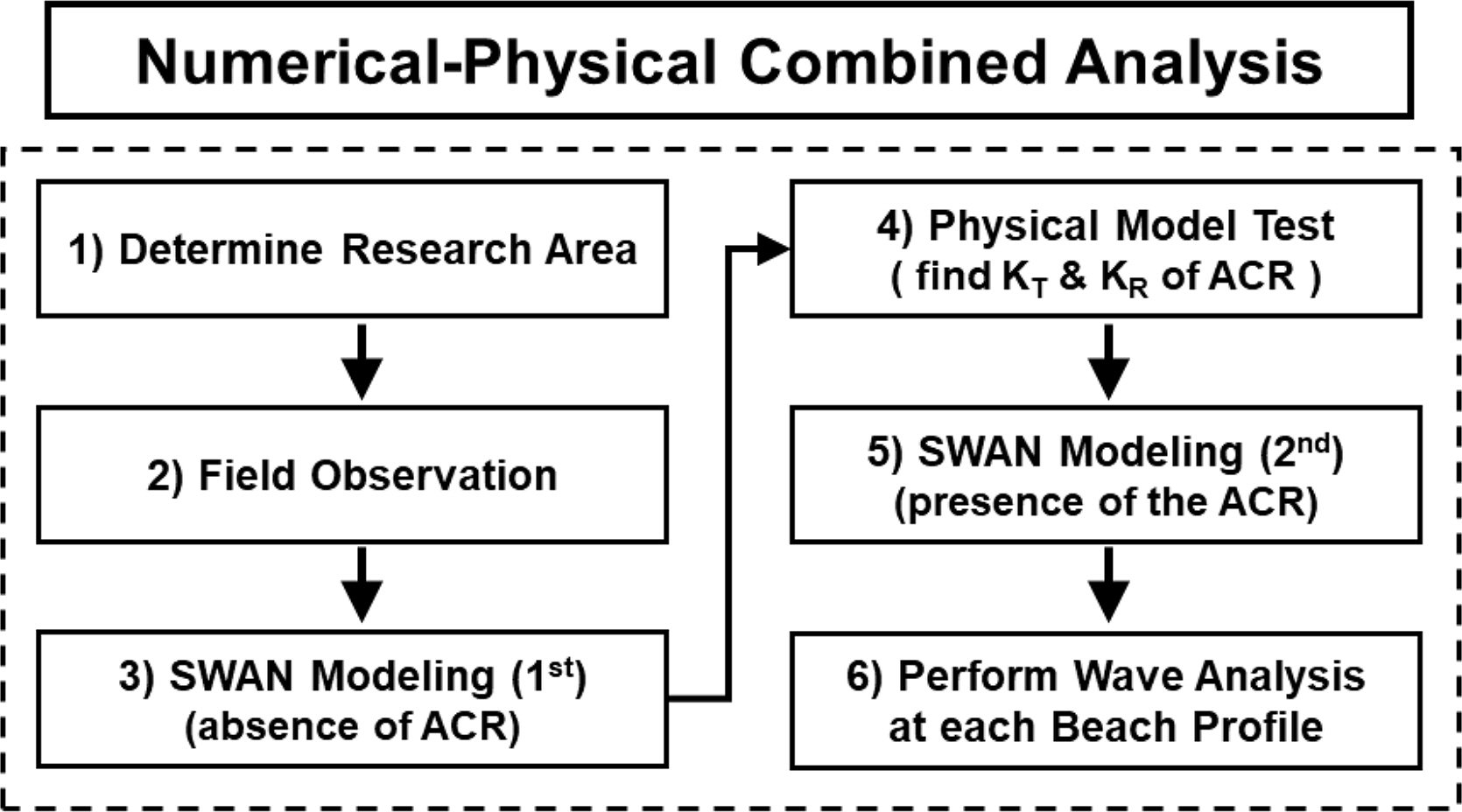
Flowchart of the research methods
2.1 Research Area: Cheonjin-Bongpo Beach, South Korea
Some beaches that had erosion issues were sampled to determine the research area. Because previous studies of ACRs did not examine the longshore current and drift, beaches with a pocket or spiral shape were preferred. Therefore, Cheonjin-Bongpo beach was used as the research area, which is denoted as ‘GW 12 littoral cell’ in South Korea. Fig. 2 shows the location of the research area.
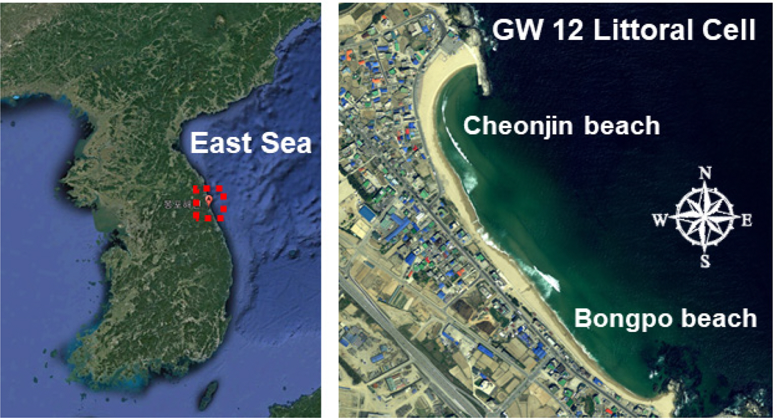
Location of Cheonjin-Bongpo beach (Google, 2005)
2.2 Field Observation
Field observations were conducted to investigate the characteristics of the research area. During the observation, echo sounder devices (Sonar-tech, AquaRuler 200S; CEE HydroSystem, CEESTAR; and VALEPORT, MIDAS) were used, and the water depth was measured until 25 m. Global Navigation Satellite System (GNSS) devices (Leica, GX1230; Leica, Viva GS16) were used to obtain shoreline data when the wave height was less than 0.7 m. The wave data were acquired using an acoustic wave and current profiler (Nortek AS, AWAC). The median grain size (D50) of the sand particle was determined to be 1.493 mm, and the calculated settling velocity was 16.7 cm/s using the van Rijn(1984)’s equation.
2.3 Application of SWAN Model
SWAN (Simulating waves nearshore) model 3rd generation was developed by Delft University of Technology (Booij et al., 1999), which aims to simulate the deformation of multi-direction irregular waves based on the wave action balance equation. The SWAN model is considered a practical method to predict wave deformation because it can consider wave reflection, diffraction, shoaling, and wave breaking. Because of these advantageous features, the 3rd generation model (Version 41.31) of SWAN based on the field observation data was used to examine the impacts of an ACR under high wave conditions. In this study, SWAN modeling was conducted with two procedures. At first, the winter wave condition for the absence of an ACR was simulated to find the incident wave height for a physical model test.
After determining both the transmission and reflection coefficient from the physical model test, second SWAN modeling was performed for both winter and summer wave conditions to examine the wave height distributions in the presence of an ACR. During SWAN modeling, the maximum wave (H1/250) was used as an incident wave for simulating the high wave condition. Moreover, bathymetry was rotated 45° counter-clockwise to perform easier modeling. Table 1 lists the specific conditions for SWAN modeling. As the SWAN model has been used widely in both the research and business practice field, an additional model verification process was omitted.
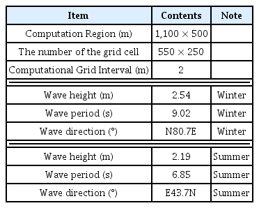
Conditions for SWAN modeling
2.4 Two-dimensional Physical Model Test and Wave Analysis
The transmission and reflection coefficient values are required as input parameters to simulate the ACR installation conditions in the SWAN model. As there was no prior research explaining the transmission and reflection coefficient according to the ACR design, a physical model test was conducted to find its values. Therefore, it was assumed that the ACR installation locations refer to the designs of a submerged breakwater in the research area from the basic plan for the 2nd coastal maintenance project (Ministry of Ocean and Fisheries, 2014). The incident wave height for the physical model was determined using both cross-sectional and planar designs for the ACR. The wave height values for the incident and transmission are located 10 m away from the ACR offshore side and 20 m away from the onshore side in the points of the prototype scale. In addition, the Froude scale with a ratio of 1 : 25 in the length scale and 1 : 5 in the time scale was applied to the physical model test. A seabed slope of 1/30 was applied because the beach slope of the east sea is generally 1/30. The capacity type of wave gauge (Kenek, CH-608E) and wave probes (Kenek, CHT-30E) were used during the physical model test. Wave calibration processes were conducted at every measuring point to obtain precise and reliable wave data. The transmission coefficient was defined as the ratio of the incident wave height (Hi ) to transmitted wave height (Ht), as shown in Eq. (1).
Healy’s formula (Healy, 1953) was applied to calculate the reflection coefficient (KR ), as shown in Eq. (2), which is based on the partial standing wave theory. To apply this equation, both the largest (Hmax) and smallest (Hmin) wave height at antinode and node of the partial standing wave, respectively, were used (see Fig. 3).
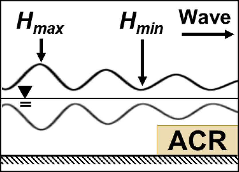
Scheme of a partial standing wave
2.5 Wave Analysis with Representative Beach Profiles
Six representative beach profile (BP1∼BP6) lines, which are the normal direction to the shoreline, were set to investigate the erosion-mitigation effects of the ACR (see Fig. 4). Generally, the trends of the wave height distribution are different between the open inlet and behind the submerged structure. In this regard, the beach profile lines were determined at the open inlet of the ACR (BP1, BP3, and BP5). Moreover, BP2, BP4, and BP6 represent the beach profile lines, which are located behind the ACR structure.
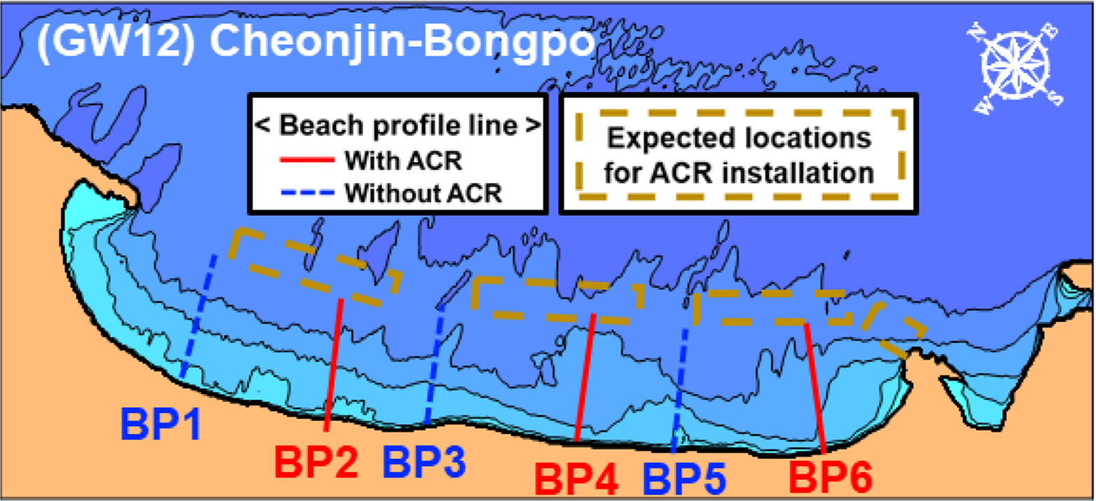
Beach profile lines (Note that BP means the Beach Profile)
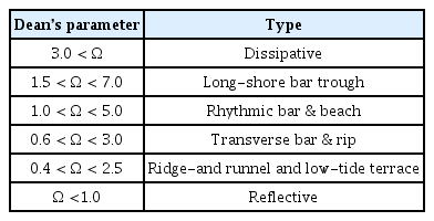
Type of beach profile based on the Dean’s parameter
With these beach profiles, the critical wave heights at each water depth condition were calculated based on the McCowan (1894)’s wave breaking parameter (κ), which has a general value of 0.78 (see Eq. (3)).
Subsequently, wave-breaking locations were determined, where the wave height value given by SWAN modeling is greater than that of the wave breaking parameter cases. The height (Hb) and depth (hb) of the breaking wave were decided. The slope for the beach profile (tanβ) was defined as an angle from the wave breaking point to the shoreline.
The Dean’s parameter (Ω) introduced by Dean (1977), mass flux (M), undertow (ub), maximum wave setup (η̄max), and surf-scaling parameter (∊s), which are relevant factors to elucidate the high wave control performance of the ACR, were computed.
3. Numerical-Physical Combined Analysis
3.1 SWAN Modeling for Incident Wave Determination
SWAN modeling was first carried out to determine the incident wave for the physical model test and examine the wave height distribution without an ACR. In this regard, the wave heights in front of three ACRs, denoted as H1, H2, and H3, were averaged (see Fig. 5). Consequently, the incident wave was determined to be 2.40 m for performing the physical model test, as shown in Table 3.
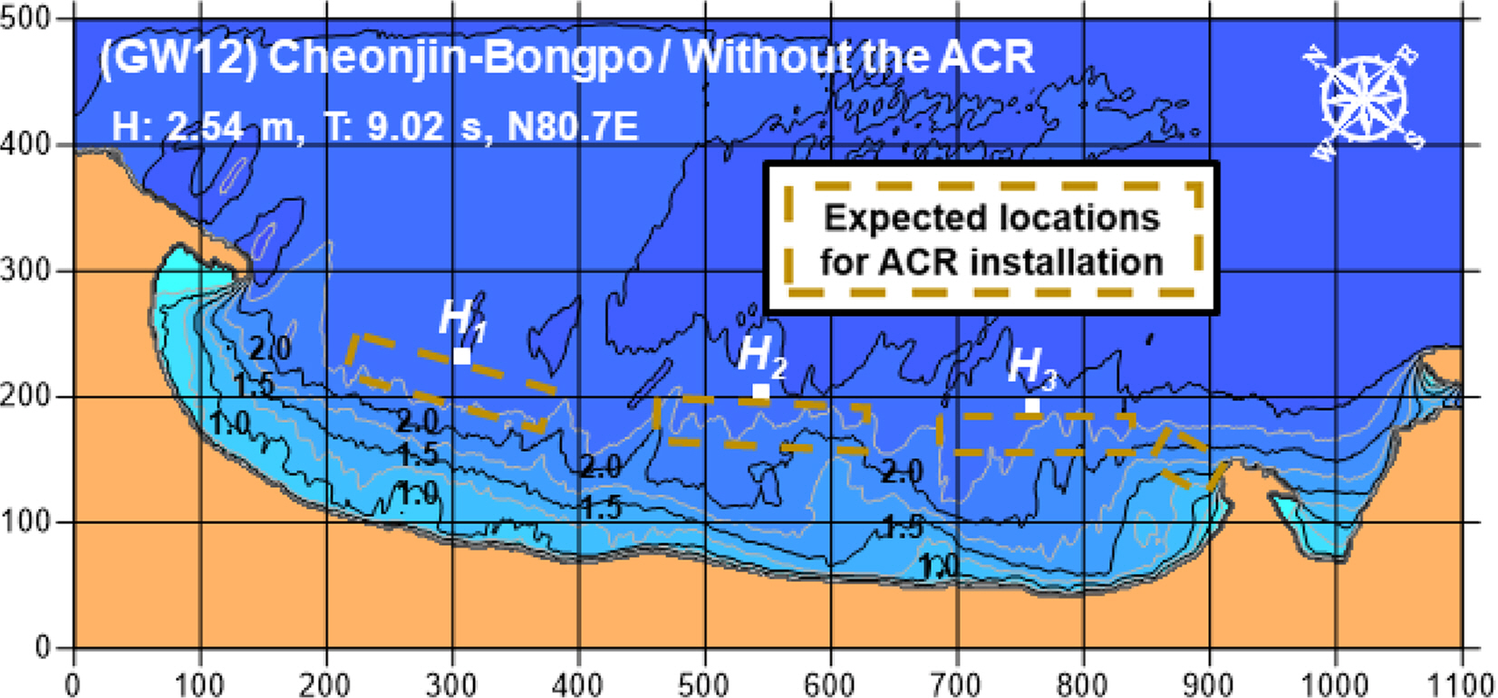
Wave height distribution (without an ACR)

Wave heights
3.2 Physical Model Test for Finding KT and KR
To determine the relevant transmission and reflection coefficient, the structure geometry and wave condition were designed based on the Froude similarity scales (Table 4). A regular wave was generated until it reproduced the target wave (H = 9.56 cm, T = 1.80 s) at the incident wave measuring point.
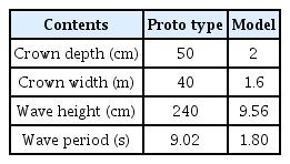
Experimental designs with the Froude scale
Fig. 6 shows the experimental design for this physical model. The incident and transmitted wave heights were measured at WP1 and WP2, respectively. Moreover, the wave measurement was conducted from 17.2 m to 23.5 m to determine both the transmission coefficient (KT) and reflection coefficient (KR).
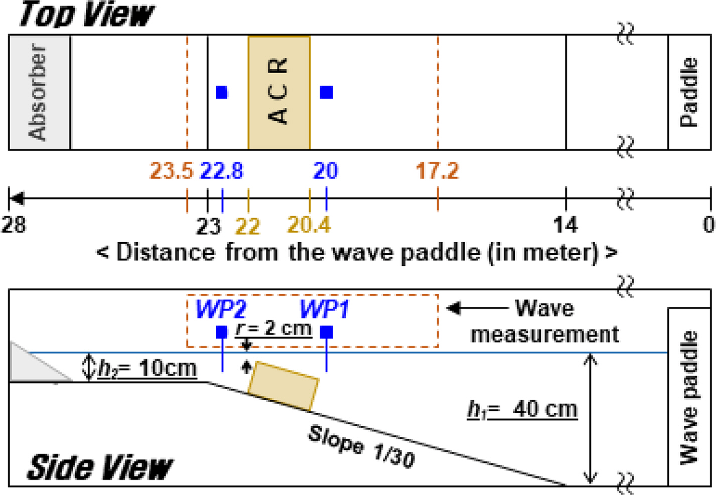
Experimental design for the physical model test
Fig. 7 shows the results of the wave measurement. The results indicate that remarkable wave attenuation occurred from the ACR. Moreover, a partial standing wave occurred in front of the ACR. In this regard, the calculated transmission coefficient (KT) was 0.36 based on the Hi (9.44 cm) and Ht (3.40 cm) values. Moreover, the calculated reflection coefficient (KR) was 0.39. These KT and KR values were applied to both the winter and summer wave simulations.
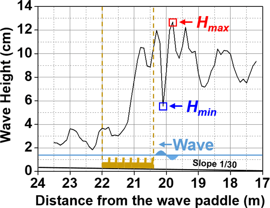
Results of wave height in the physical model
4. Impacts of the ACR Installation on Wave Control
4.1 Trends of Wave Height Reduction and Wave Breaking
The second SWAN modeling was performed to investigate the wave height distribution trends with ACR installation for winter and summer wave conditions. Fig. A1 provides detailed information on the ACR structure. Fig. 8 shows the wave height distribution results in the presence of the ACR for a winter wave.

Wave height distribution (with an ACR)
Table 5 lists the wave height percentile in the presence and absence of an ACR case calculated at each beach profile line. The results of significant wave reduction indicate that ACR installation plays a crucial role in wave attenuation at the rear side of its structure for both winter and summer cases. Moreover, greater wave height mitigation (58.95∼70.90%) occurred in the presence of an ACR, whereas no significant wave reduction occurred without ACR installation (83.95∼96.15%).
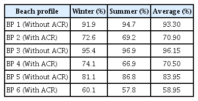
Wave height ratio for each wave profiles
The wave breaking trends also differed according to the ACR installation. Fig. 9 shows the wave-breaking height and wave-breaking distance from the shoreline. In the case of ACR installation, waves with smaller heights break near the shoreline, whereas relatively larger waves break further from the shoreline. The ACR induced breaking for larger waves in advance, allowing only smaller waves to propagate over the ACR. A significant difference was not observed between the winter and summer high waves, which means that the ACR plays a positive role in terms of wave height reduction.

Wave breaking trends at each beach profile according to ACR installation
4.2 Impacts of Wave-induced Nearshore Current
The mass flux (M), undertow (ub), and maximum wave setup (η̄max) at each beach profile were calculated and compared to investigate the impacts of wave-induced current. Table 6 lists the computed values of M, ub, and η̄max . According to average values for the winter and summer results, smaller mass flux (∼50%), undertow (∼80%), and wave set up values (∼61%) were observed with ACR installation, highlighting the positive impacts on shoreline stability.

Computed values related to the nearshore current
4.3 Application of Morpho-dynamic Parameter for Wave Analysis
As a wave is a key parameter that determines the shape of the shoreline, the Dean’s parameter (Ω) and surf-scaling parameter (∊s) were computed to determine the impacts of the waves in terms of shoreline changes (Table 7 and Table 8). Under winter and summer high wave conditions, the Dean’s parameter decreased in the ACR cases, which is closer to the reflective wave type compared to the dissipation wave type.

Dean’s parameter (Ω) for each beach profile

Surf-scaling parameter (∊s) for each beach profile
When waves propagate over the ACR, a decrease in surf-scaling parameters usually occurs, particularly in BP2, BP4, and BP6, suggesting that wave-induced erosion can be mitigated. Moreover, the planar design of the ACR suggested in this study appears to be more effective for summer waves (improved in six beach profiles) than winter waves (improved in four beach profiles) in terms of high wave control. Overall, an ACR can mitigate erosion caused by high waves.
5. Conclusions
To investigate the feasibility of an artificial coral reef (ACR) as a coastal erosion prevention method, a case study was conducted by performing field observations and the numerical-physical combined method for Cheonjin-Bongpo Beach in South Korea. The main results of this research can be summarized as follows.
The calculated wave transmission and reflection coefficients of the ACR were 0.36 and 0.39, respectively, based on the 1/25 Froude scale of the physical model test.
Remarkable and greater wave height reduction (58.95∼70.90%) occurred in each beach profile with ACR installation, whereas no significant wave height attenuation took place for the absence of ACR cases (83.95∼96.15%). In addition, under the ACR installation condition, small waves break near the shoreline, but larger waves break far from the coast.
In the presence of an ACR, the mass flux (M), undertow (ub), and maximum wave setup (η̄max) were smaller than in the absence of an ACR. This suggests that an ACR plays a remarkable role in mitigating wave-induced current.
When an ACR was applied to the research area, both the Dean’s parameter (Ω) and surf-scaling parameter (∊s ) decreased. Therefore, a wave with the dissipative property changed to the reflective or intermediate type, which plays a positive role in erosion mitigation from high waves. In addition, the planar design for the ACR applied in this study showed greater wave control performance than the winter wave condition.
Because of the complicated coastal process and uncertainty of irregular waves, further studies will be needed to verify the feasibility of an ACR and consider more wave conditions. Furthermore, this model should be applied to other research areas.
Acknowledgements
The authors thank Professor Jung Lyul Lee of Sungkyunkwan University for sharing his valuable knowledge and insights that encourage us to conduct this research.
Notes
This research was a part of the project titled ‘Practical Technologies for Coastal Erosion Control and Countermeasure’, funded by the Ministry of Oceans and Fisheries, Korea. (20180404)
References
Appendices
Appendix Fig. A1 Dimensions and formation of the ACR structure.
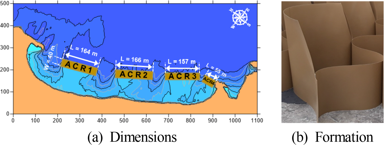
Detail information of the ACR structure