Higher-order Spectral Method for Regular and Irregular Wave Simulations
Article information

Abstract
In this study, a nonlinear wave simulation code is developed using a higher-order spectral (HOS) method. The HOS method is very efficient because it can determine the solution of the boundary value problem using fast Fourier transform (FFT) without matrix operation. Based on the HOS order, the vertical velocity of the free surface boundary was estimated and applied to the nonlinear free surface boundary condition. Time integration was carried out using the fourth order Runge–Kutta method, which is known to be stable for nonlinear free-surface problems. Numerical stability against the aliasing effect was guaranteed by using the zero-padding method. In addition to simulating the initial wave field distribution, a nonlinear adjusted region for wave generation and a damping region for wave absorption were introduced for wave generation simulation. To validate the developed simulation code, the adjusted simulation was carried out and its results were compared to the eighth order Stokes theory. Long-time simulations were carried out on the irregular wave field distribution, and nonlinear wave propagation characteristics were observed from the results of the simulations. Nonlinear adjusted and damping regions were introduced to implement a numerical wave tank that successfully generated nonlinear regular waves. According to the variation in the mean wave steepness, irregular wave simulations were carried out in the numerical wave tank. The simulation results indicated an increase in the nonlinear interaction between the wave components, which was numerically verified as the mean wave steepness. The results of this study demonstrate that the HOS method is an accurate and efficient method for predicting the nonlinear interaction between waves, which increases with wave steepness.
1. Introduction
High-precision wave prediction technology is imperative for both the design of ships and offshore structures to be operated at sea and also for their maintenance. Because ocean wave have nonlinear characteristics, a broad understanding of waves and highly precise numerical techniques are required to accurately predict their generation and propagation.
The numerical technique for predicting waves is mainly the efficiency analysis based on potential flow. There are two methods to reflect the nonlinear boundary conditions of the free surface. One is a higher-order analysis method base on the perturbation method, and another one is mixed Eulerian-Lagrangian (MEL) methods (Longuet-Higgins and Cokelet, 1976) using a completely nonlinear free surface condition.
In particular, the MEL method, which is flexible for the analysis of the strong nonlinearity of free surface and wave-body interactions, was applied using various solution methods of the Laplace equation such as boundary element method (BEM), finite element method (FEM), and harmonic polynomial cell (HPC) (Longuet-Higgins and Cokelet, 1976; Wu et al., 1998; Shao and Faltinsen, 2014). Because the mentioned solution method of the Laplace equation inevitably requires matrix operation, the MEL method, which reconstructs the free surface grid every time step to reflect the completely nonlinear free surface, requires high computational costs for calculations of a solution of boundary value problem(Oh et al, 2018). In contrast, the higher-order spectral (HOS) method of Dommermuth and Yue (1987), based on a higher-order analysis method, can determine the solution of the boundary value problem using the fast Fourier transform (FFT) without a matrix operation. Therefore, compared to the MEL-based analysis method, this method is significantly more computationally efficient (Kim, 1993). Therefore, the HOS method is widely used for predicting the propagation and generation of nonlinear waves (Ducrozet et al., 2016). Owing to the recent developments in computing equipment, computational fluid dynamics (CFD) is being increasingly used for analyzing loads and the behaviors of offshore structures. However, the direct CFD simulation for irregular sea state requires high computational cost, and cumulative error due to long-time simulation is inevitable. Currently, studies on the potential flow method and CFD coupling are actively being conducted to address this challenge and generate efficient and highly precise irregular wave predictions. In particular, the HOS method is known to be one of the best methods for CFD coupling in terms of high accuracy and computational efficiency (Gatin et al., 2017). Therefore, it is expected that the development of a wave simulation code via the HOS method can be widely used for both the nonlinear wave prediction study and the efficient implementation of the CFD wave field.
Because boundary conditions except that of the free surface cannot be defined, it is challenging to generate waves like a wave tank using the conventional HOS method. Under the nonlinear free surface conditions, it is necessary to fine-tune the results of repetitive calculations because the transfer function can only be calculated under the linear free surface conditions although waves can be generated via the disturbance of the free surface. Therefore, to work on the boundary condition for the wave generation, Kim (1993) introduced the boundary element method to the HOS method while Bonnefoy et al. (2006) worked on the boundary condition for the wave generation using the pseudo-spectral basis of the cosine function and an additional potential technique. The aforementioned methods are cumbersome because they require the introduction of a separate additional boundary value problem. Recently, Liam et al. (2014) applied a nonlinear adjustment zone to the analytic and variational Boussinesq models to successfully transform the linear wave generated in the free surface into a nonlinear wave, which is expected to be applied to the HOS model.
In this study, a nonlinear wave simulation code using an efficient HOS method was developed. According to the expansion of Dommermuth and Yue (1987), the vertical velocity of the free surface boundary, which depends on the HOS order, was estimated and applied to the nonlinear free surface boundary condition. Time integration was performed using the fourth order Runge–Kutta method, which is known to be stable against the nonlinear free surface problem. The zero-padding method was used to secure numerical stability against the aliasing effect (Canuto et al., 1988). The nonlinear adjustment region (Liam et al., 2014) and wave damping zone were introduced for the simulations of wave generation. The adjusted simulation of Dommermuth (2000) was performed and compared with the eighth order Stokes theory to verify the developed code. The long-time simulation was performed on the irregular wave distribution to determine the characteristics of nonlinear wave propagation. Nonlinear adjustment and damping zones were introduced to implement a numerical wave tank, thus confirming that a nonlinear regular wave was successfully generated. As the mean wave steepness increased, the nonlinear interaction between wave components was numerically evaluated by simulating the generation of irregular waves based on the mean wave steepness in the numerical wave tank.
2. Mathematical Formulation and Numerical Technique
2.1 Mathematical Formulation
In this study, a rectangular fluid domain with a horizontal length L and constant depth h was considered in a Cartesian coordinate system. In this coordinate system, the mean water surface was on the x-axis while the vertical z-axis was directed upwards. Assuming that the fluid is incompressible and inviscid and the flow is irrotational, the velocity of the fluid defined as the gradient of the velocity potential ϕ and the continuity equation, which is the governing equation, is transformed into the Laplace equation as expressed in Eq. (1).
Using the surface potential φs, the kinematic boundary conditions and dynamic boundary conditions of the free surface can be expressed by Eqs. (3)–(4).
The vertical velocity W can be calculated using the HOS model presented by Dommermuth and Yue (1987) and West et al. (1987). The free surface ζ and surface potential φs based on to time progress can be obtained by integrating Eqs. (3)–(4), which substitutes the calculated vertical velocity W. It is assumed that the horizontal region is infinite in the HOS model and the periodic boundary condition is adopted as expressed in Eq. (6).
The velocity potential, which is the solution of the Laplace equation that satisfies the aforementioned free surface boundary condition (Eqs. (3)–(4)), lateral periodic boundary condition (Eq. (6)), and bottom boundary condition (Eq. (7)), can be defined by Eq. (8) using a Fourier pseudo-spectral basis.
Similar to the velocity potential, the surface potential φs and free surface ζ can be defined by a Fourier pseudo-spectral basis as expressed in Eqs. (10)–(11).
The vertical velocity W can also be expressed with perturbation expansion as in Eq. (14), as presented in Eq. (12).
The perturbation vertical velocity W(m) in Eq. (15) was calculated via the perturbation velocity potential ϕ(m), which can be used to measure the vertical velocity W at ζ using Eq. (14).
2.2 Numerical Technique
In this study, the free surface ζ and surface potential φs can be predicted depending on time integration using Eqs. (3)–(4), which define the boundary conditions of the free surface. As for time integration, the fourth order Runge–Kutta method, which ensured stability, was adopted as presented by Dommermuth and Yue (1987). The physical quantity and vertical velocity W of the spatial differential included in the boundary condition of the free surface were calculated by applying the FFT algorithm. In this study, a numerical technique was implemented using MATLAB (Matrix laboratory). Because it supports the FFT algorithm and multi-thread, MATLAB provides fast computation. Regarding the HOS method, the multiplication of the nonlinear free surface boundary conditions was performed in a physical space rather than a spectra space. Although such transformation is efficiently performed using FFT, it leads to an aliasing phenomenon. It is therefore imperative to clearly eliminate the aliasing phenomenon to ensure the stability of the analysis owing to its influence on numerical stability. In this study, the zero-padding method was used to eliminate the aliasing phenomenon. Zero padding is a method for performing multiplication operations without aliasing in the physical space by filling in zero to expand the spectral space prior to multiplication. This is accompanied by the expansion of the spectral space, leading to an increase in computational cost as the consequence of an increase in the calculation domain. Therefore, appropriate spatial expansion was achieved via the half-rule as expressed in Eq. (16) (Canuto et al., 1988; Gatin et al., 2017).
The analysis of the HOS simulation is generally performed from the initial conditions of free surface ζ and surface potential φs at the free surface, in which the initialization is known to have significant influence on the numerical stability. According to the study by Dommermuth (2000), the simulation of the HOS method under the linear initial condition causes numerical instability because it does not satisfy the nonlinear free surface boundary conditions in Eqs. (3) and (4). Therefore, Dommermuth (2000) proposed an adjustment scheme to initiate the linear initial condition to the nonlinear free surface condition. This scheme enables the smooth transformation of the nonlinear solution via the relaxation of the nonlinear term of the free surface against time. Eqs. (17)–(18) express the free surface condition to which the relaxation of the nonlinear term was applied by introducing the relaxation time Ta and relaxation index n proposed by Dommermuth (2000).
In this study, the linear free surface ζ1st and linear potential ϕ1st were adopted as the initial conditions of the regular wave under deep sea conditions, as expressed in Eqs. (19)–(20).
By substituting the calculated wave amplitude Ai into Eqs. (22)–(23), the initial conditions for the irregular wave simulation, ζirregular and φirregular can be calculated.
3. Numerical Simulation
Numerical tests were performed to verify the HOS code developed in this study and to observe related characteristics. An analysis of linear single waves was performed to verify the HOS code, whereas a numerical analysis of the irregular wave field implemented was performed using the JONSWAP spectrum defined above to understand the developed HOS code characteristics.
3.1 Adjusted Simulation of Single Wave
According to the study by Dommermuth (2000), when a linear solution is used as the initial condition and relaxation is applied to the HOS method for a certain period of time, it adjusts to a nonlinear solution. Dommermuth (2000) performed an adjustment simulation at a wave steepness of kA = 0.1 and presented the convergence result of the eighth harmonic component of the Stokes wave. In this study, the developed code was verified by performing calculation conditions, as presented in Table 1, which are the same conditions as those of Dommermuth (2000); after that, the results were compared.

Calculation conditions for adjusted simulation
Similar to the study by Dommermuth (2000), a single wave adjustment simulation was performed using 64 modes for 200 seconds with a time step Δt at 0.025 intervals. In the HOS simulation, the linear solution converged to a nonlinear Stokes wave, as illustrated in Fig. 1.
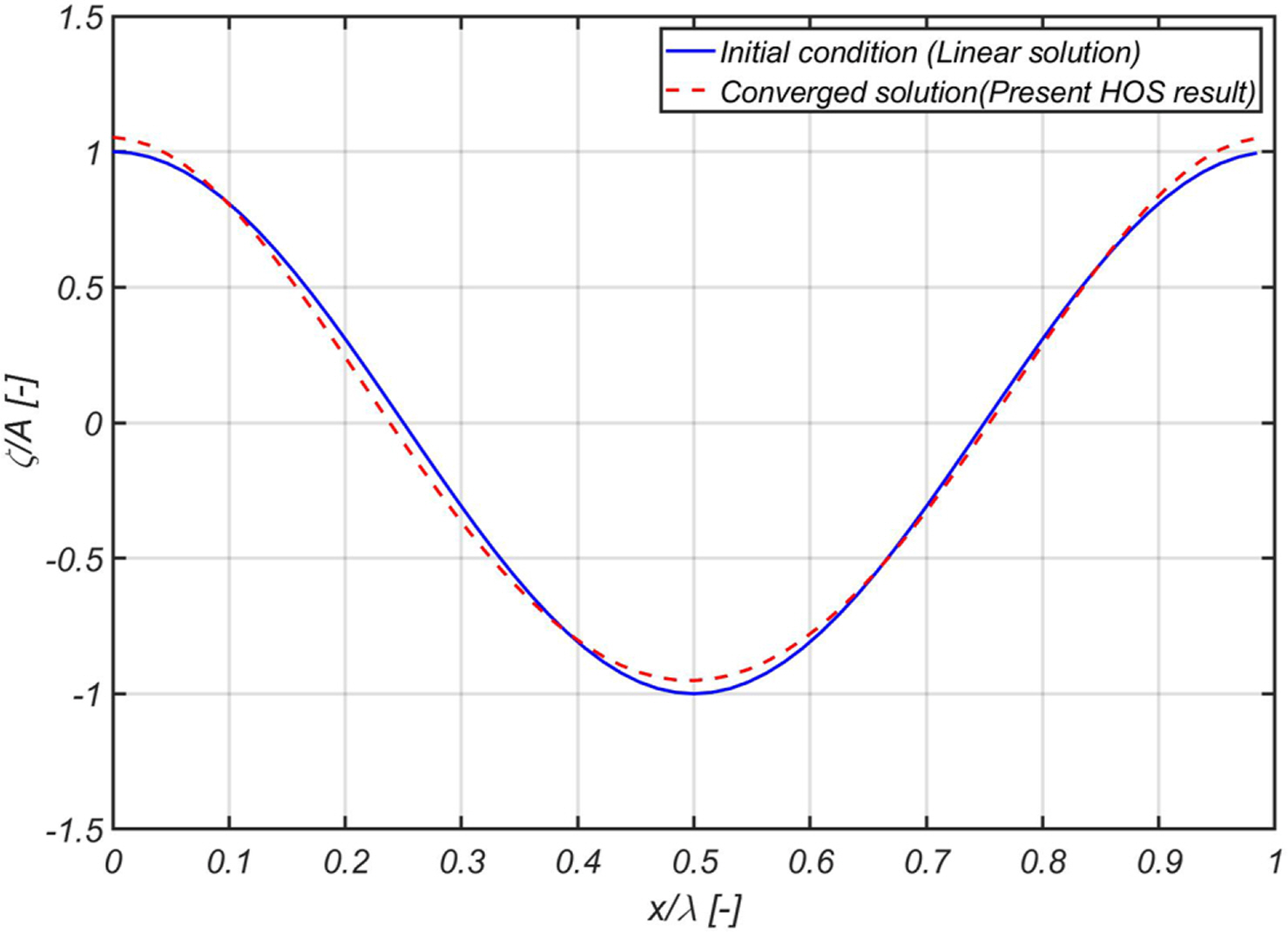
HOS result of monochromatic Stokes wave
It was determined that the eight harmonic components of the eighth order Stokes wave converged over time and that the convergence pattern of each harmonic component was similar to the results obtained by Dommermuth (2000), as illustrated in Fig. 2.

Adjusted simulation results for monochromatic Stokes wave
The converged results were compared with the analysis solution, as well as the results obtained by Dommermuth (2000), as presented in Table 2. Compared to the analysis solution, it was inferred that the relative error of the code developed in this study was insignificant at less than approximately 0.1%. The validity of the developed code was verified via this result.
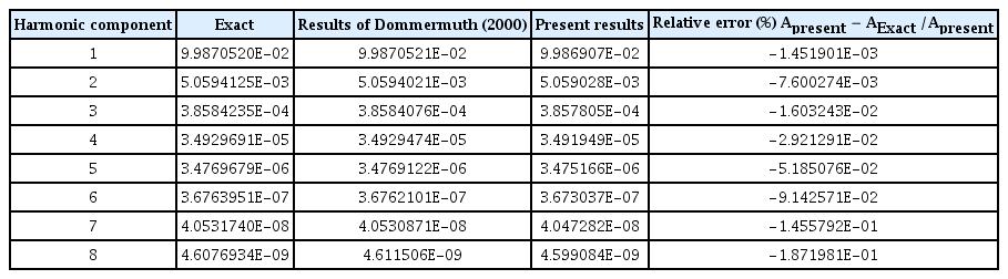
Comparison of harmonic amplitudes of Stokes wave
3.2 Irregular Wave Simulation
An irregular wave simulation was performed to understand the characteristics of the HOS method. Analysis conditions were defined with reference to the analysis case of Ducrozet et al. (2016), as presented in Table 3. The corresponding condition was a mean steepness of (

Calculation conditions for irregular wave simulations
The initial conditions of the irregular wave for this case can be created using Eqs. (22)–(23), as illustrated in Fig. 3(a).
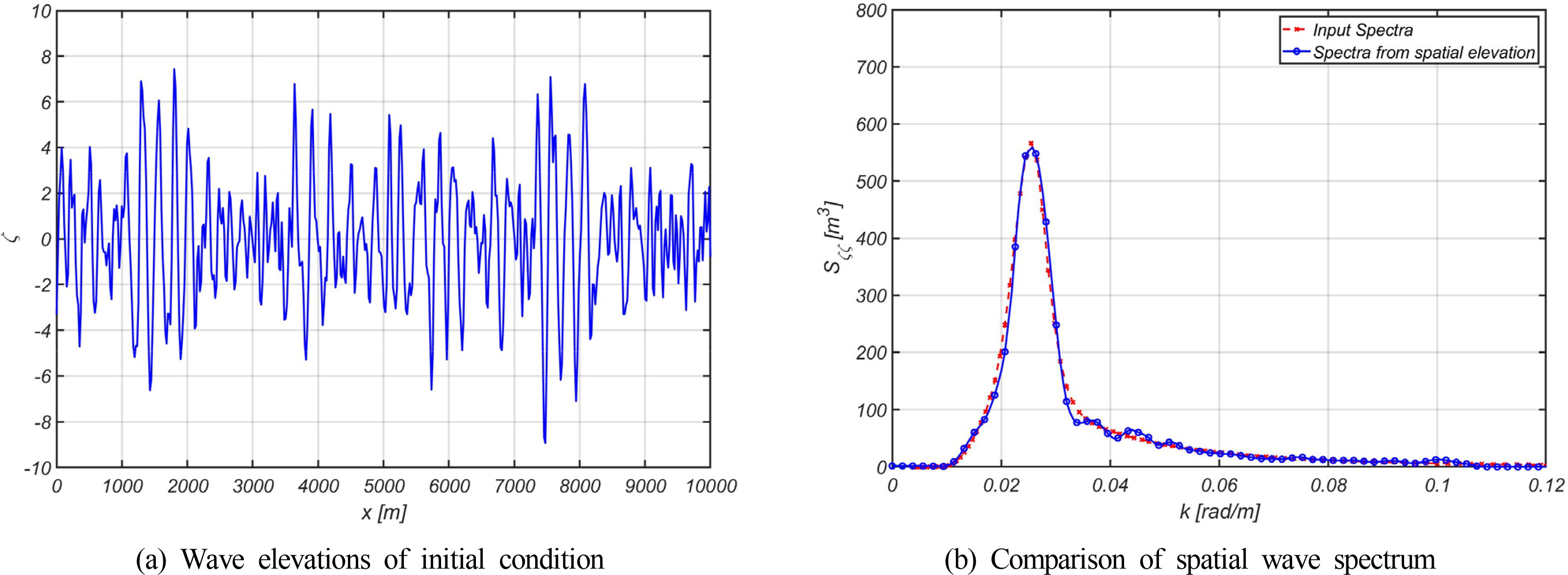
Initial condition of irregular wave simulations
The spatial wave spectrum, obtained from the wave distribution generated, and the input wave spectrum were compared, as illustrated in Fig. 3(b). The two spectra exhibited satisfactory agreement, thus validating the generated wave distribution. The boundary condition at both ends was periodic and the wave from 10 000 m was re-introduced at 0 m when the simulation was performed. Therefore, the HOS method can efficiently simulate the development of irregular waves over a long period of time within a limited spatial grid.
In this study, simulation was performed by varying the order M to 1, 3, 5, and 8 for the same initial condition. Fig. 4 presents the normalized maximum wave height and kurtosis (κ) based on the change in time. When the normalized maximum wave height exceeds 2 m, it is called an abnormality index (AI). It is known that the abnormality index and kurtosis are highly correlated with the occurrence of Freak wave (Kim, 2019). The abnormality index was calculated using Hmax and H1/3 was determined via the zero crossing analysis of the wave distribution at every time step. The kurtosis was a measure adopted to statistically establish the difference with the normal distribution, as defined in Eq. (25).
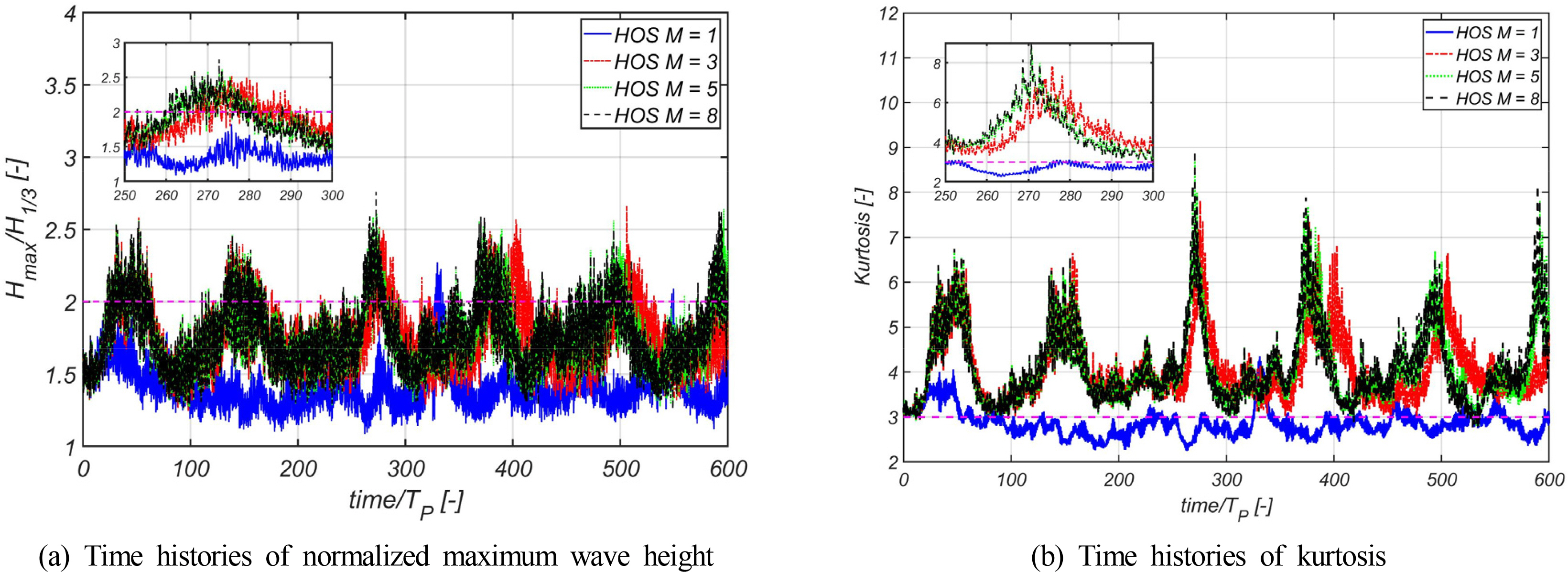
Evolution of normalized maximum wave height and kurtosis
The spatial wave spectrum was compared at the final time step, as illustrated in Fig. 5(a). The spectrum represents the distribution of energy, and the change in the spectrum indicates the change in energy distribution. Therefore, from the change in the magnitude of the spectrum of the corresponding wave number, it can be inferred that it was redistributed to the energy of other wave numbers. In the linear free surface boundary condition of order 1, it was concluded that the spatial wave spectrum is approximately similar to the initial value, thus indicating that the energy distribution between the components of the wave remains unchanged. However, the spatial wave spectra of orders 3, 5, and 8 exhibited different results from the initial values. This could be attributed to the nonlinear interaction between the wave components owing to the nonlinear free surface boundary condition, subsequently, it can be inferred that the wave energy was redistributed between the wave components. The wave displacement over time at the center point of the simulation domain was transformed into a spectrum, as illustrated in Fig. 5(b). It was similar to the initial value in the calculation condition of order 1, thus indicating the absence of interactions between wave components. However, the wave spectrum was different from the initial spectrum under the calculation conditions of orders 3, 5, and 8, which is also attributed to the nonlinear interaction between the wave components, and allows us to infer that the energy between the wave components was redistributed. From these results, it was determined that the irregular wave simulation using the HOS method is a satisfactory numerical tool for observing the nonlinear interaction between wave components. As earlier mentioned, it was concluded that the conventional HOS method has the advantage of the long-time simulation for the initial conditions given as periodic boundary conditions at both ends. However, there are limitations to this simulation in that waves are generated only in a limited space and at a specific point, such as in a test tank. A separate numerical technique is required to generate and simulate waves as in a test tank. In the following chapter, a numerical technique for the simulation of wave generation is described. The technique was verified and its characteristics were identified via numerical tests.
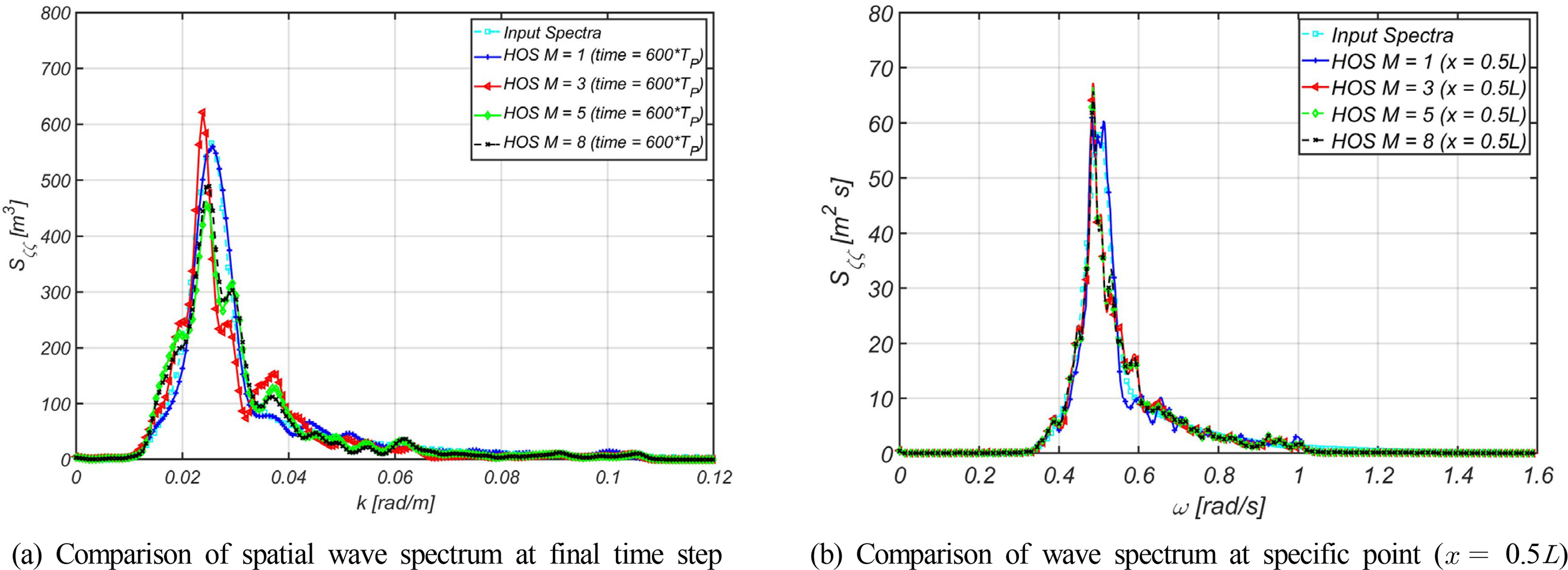
Wave spectrums of irregular simulations
4. Numerical Technique and Numerical Simulation for Wave Generation
4.1 Numerical Techniques for Generating Waves
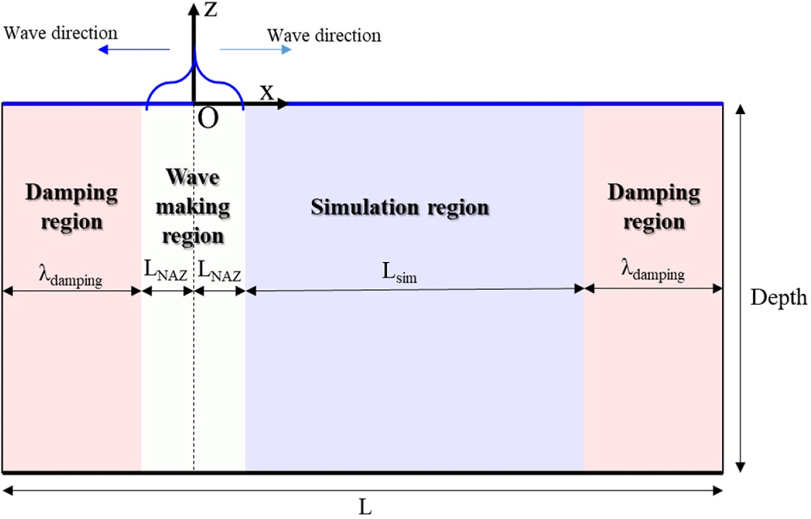
Because boundary conditions are undefined except those of the free surface, the conventional HOS method has limitations in implementing the boundary conditions of the piston- or flap-type wave maker, such as a traditional wave tank. Tuning through repetitive calculations is required because wave generation owing to the forced disturbance of free surface can be represented in a transfer function under linear free surface conditions alone and cannot be represented under nonlinear free surface conditions. Therefore, Kim (1993) applied the wave generation technique based on the submerged circular cylinder by merging the HOS method and the boundary element method, whereas Bonnefoy et al. (2006) adopted the pseudo-spectral basis of the cosine function and the additional potential technique to include the boundary condition for the wave generation unlike in the conventional HOS method. In this study, the feasibility of nonlinear wave generation was investigated via the forced disturbance of free surface using the wave transfer function at specific wave generation points unlike in the studies conducted by Kim (1993) and Bonnefoy et al. (2006). As earlier mentioned, the wave transfer function via the forced disturbance of free surface is only feasible under linear free surface conditions. Therefore, to make the wave transfer function possible in the nonlinear free surface, the nonlinear adjustment zone applied to the analytic and variational Boussinesq models by Liam et al. (2014) was introduced to the HOS method, as illustrated in Fig. 6. To prevent the inflow of waves owing to the periodic conditions at both ends, a damping zone was also applied, as illustrated in Fig. 6.

Nonlinear adjustment and damping zone
The nonlinear adjustment zone plays a role similar to the aforementioned adjustment scheme presented by Dommermuth (2000). The nonlinear term of the free surface boundary condition degrades the simulation stability of wave generation for wave disturbances at a specific wave generation point. Therefore, similar to scheme of Dommermuth (2000), which weakens the effect of nonlinear terms against time, it is necessary to mitigate the effect of nonlinearity on spaces. The study on the nonlinear adjustment zone in Section 3.2 was conducted by Liam et al. (2014) and it was inferred that a larger adjustment interval LNAZ was required as the wave steepness increased.
The nonlinear adjustment zone is defined as a function of distance, as expressed in Eq. (26). The damping zone was applied to the boundary of both ends, as illustrated in Fig. 6. This was done to prevent the inflow and outflow of waves through the boundary owing to the periodic boundary conditions at both ends. The damping zone was applied to the physical quantity of each boundary condition, as expressed in Eq. (27).
Wave disturbances for wave generation were performed at the point where x was equal to zero, and the wave transfer function was calculated using the harmonic simulation results of white noise under the boundary condition of the linear free surface, as illustrated in Fig. 6.
4.2 Wave Generation Numerical Simulation
The wave generation simulation of regular and irregular waves was performed to verify and analyze the characteristics of the numerical technique for wave generation earlier described. The analysis was performed in the same calculation domain as in Fig. 7 under the calculation conditions presented in Table 4.
Calculation domain for wave generation simulation
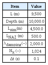
Calculation conditions for the wave generation simulation of regular and irregular waves
A wave transfer function can be created via the harmonic simulation results of white noise for the corresponding conditions, as illustrated in Fig. 8. ζinflux denotes the disturbance amplitude of the wave at the point where x = 0.

Wave transfer function for specific calculation condition
The wave generation simulation of regular waves was performed under the conditions of wave steepness, where k A was 0.025 and 0.126. The simulation that did not apply the nonlinear adjustment zone was additionally performed to understand the characteristics of the technique.
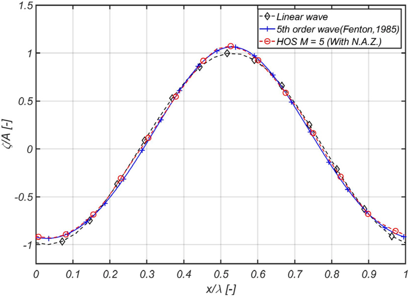
It was deduced that when kA is 0.025, it indicates the condition for generating waves with weak nonlinearity, where the amplitude difference between orders 1 and 5 is insignificant, as demonstrated in Fig. 9(a). In contrast, the condition when kA is 0.126 indicates the generation of waves with strong relative nonlinearity, which shows nonlinear characteristics with a high crest and steady trough, as demonstrated in Fig. 9(b). To strictly observe these nonlinear characteristics, it was compared with the 5th order Stokes wave (Fenton, 1985), as illustrated in Fig. 10. It was inferred that the shape of the generated wave did not only agree well with the 5th order Stokes wave, but also the waves of desired periods and amplitudes can be generated via the wave transfer function determined in advance, as demonstrates in Fig. 8. Regarding the application of nonlinear free surface boundary conditions without the nonlinear adjustment zone, the amplitude and phase of the wave differed from the linear result when kA was 0.025, and the simulation of regular wave generation diverged when kA was 0.126, as illustrated in Fig. 9(a). Consequently, it was concluded that it is necessary to apply a nonlinear adjustment zone when simulating wave generation via wave disturbance. It was determined that the HOS-based numerical harmonic tank can be implemented using a numerical technique such as nonlinear adjustment and damping zones based on the above results.
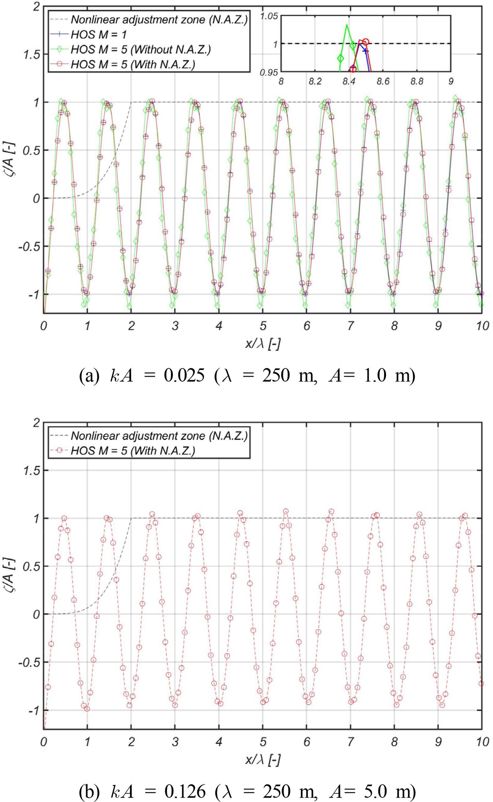
Regular wave making simulations
Comparison of steep wave simulation (kA = 0.126)
In the same calculation condition as the regular wave, the simulation of the irregular wave was performed for the irregular wave condition in Table 5. To observe the nonlinear effect according to the increase in the significant wave height, the simulation was performed under the three conditions of the mean wave steepness (

Calculation conditions for irregular wave simulation
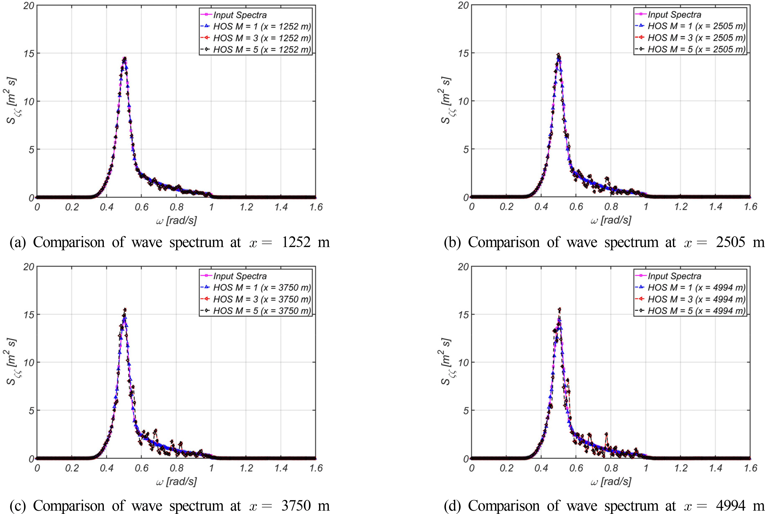
For comparison, the random phase was used identically in all simulations when generating irregular waves. After the relaxation distance of the nonlinear adjustment zone, a spectral analysis was performed on the wave time series at 4 points (x = 1252 m, 2505 m, 3750 m, and 4994 m).
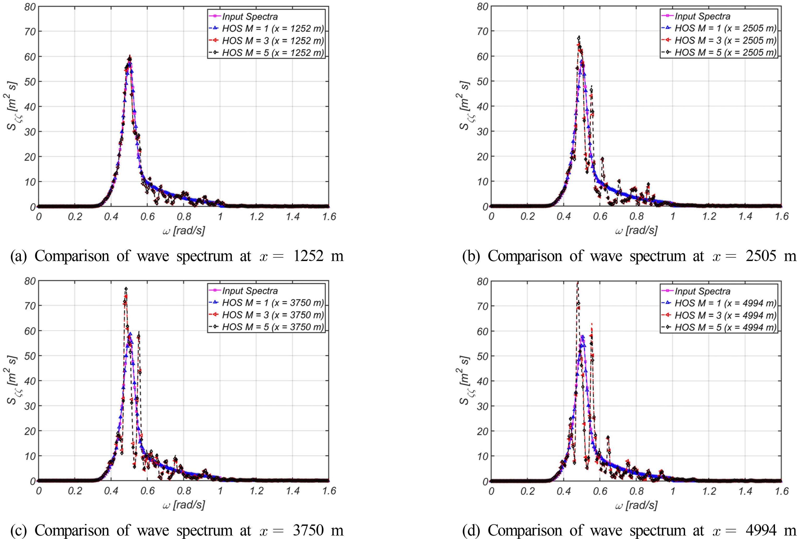
Fig. 11 illustrates the mean wave steepness of 0.01. It was determined that the spectrum of 4 points almost coincide with no difference depending on the HOS order, and also that the spectrum of 4 points almost coincide with the spectrum input when generating the wave. It can be inferred that energy was not redistributed between frequencies because there was an insignificant nonlinear interaction between wave components during the generation and propagation of irregular waves. This means that the nonlinearity that appeared was insignificant owing to the low mean wave steepness of the calculation condition. Fig. 12 illustrates the mean wave steepness of 0.05. Except for the case of order 1, it was determined that the difference in the input wave spectrum increased with an increase in the distance from the origin, which is the wave generation point. This indicates that the energy distribution between frequencies was insignificant owing to the nonlinear interaction between wave components during wave propagation as earlier mentioned. Because the results of orders 3 and 5 are almost identical, it can be inferred that nonlinear interactions can also be reflected at order 3 when the mean wave steepness is 0.05. Fig. 13 presents the results of mean wave steepness at 0.1. It’s similarity to the input wave spectrum was apparent when x was equal to 1252 m, which is the closest point after the relaxation distance of the nonlinear adjustment zone during wave generation; however, the difference in the input wave spectrum increased as the wave propagated away from the origin of wave generation. Consequently, it can be inferred that the nonlinear interaction of the wave increased compared to the previously described wave steepness condition. Based on the comparison with the mean wave steepness of 0.05, it was deduced that the energy redistribution between wave components was more significant owing to the nonlinear interaction between wave components during wave propagation. Some differences between the results of orders 3 and 5 were determined, thus indicating that for the mean wave steepness of 0.1, nonlinear interactions can be fully reflected only when the order is considered to be 5 or above similar to the results of the irregular wave simulation in Section 3.2.

Irregular wave simulations for mean steepness smean = 0.01 (Hs =1.1 m)
Irregular wave simulations for mean steepness smean = 0.05 (Hs =5.5 m)
Irregular wave simulations for mean steepness smean = 0.1 (Hs = 11.0 m)
5. Conclusion
In this study, a nonlinear wave simulation code was developed using an efficient HOS method. Because it can determine the solution of the boundary value problem using FFT without matrix computations, the HOS method is extremely efficient in its computation compared to other free-surface numerical techniques. The vertical velocity W was estimated based on the HOS order according to the expansion presented by Dommermuth and Yue (1987). Furthermore, the time integration for the nonlinear free surface boundary condition was stably performed using the Runge-Kutta 4th order method accordingly. The aliasing phenomenon caused by the multiplication of the nonlinear free surface boundary condition was eliminated using the zero padding method, thus securing numerical stability. The conventional HOS method is limited in its simulation of wave generation in a confined space, such as in a tank, with lateral periodic conditions. Therefore, in this study, a nonlinear adjustment and damping zones were introduced to implement a numerical tank capable of generating waves via surface disturbance. Several numerical simulations were performed using the developed code, therefore, the following conclusions were derived based on the results of performed simulations:
By performing the same nonlinear relaxation simulation as in the study by Dommermuth (2000), it was inferred that the linear solution converged to the eighth order Stoke wave solution. The HOS code developed in this study was verified by demonstrating that the convergence pattern was the same as that of Dommermuth (2000) and the convergence result was highly consistent with the analysis solution.
The abnormal index and kurtosis over time were observed via the simulation of an irregular wave field with a mean wave steepness of 0.1. A high correlation between the two physical quantities was determined based on the similarity of the time series development pattern between the abnormality index and kurtosis, which are known to exhibit high correlation with the occurrence of freak waves. It was inferred that to fully reflect the nonlinear interaction between waves in this mean wave steepness 0.1, order 5 or above needs to be considered.
In the simulation of an irregular wave field, it was determined that the difference between the wave spectrum given as the initial condition and that of the final time step increased as the order increased. It was therefore concluded that energy was redistributed between wave components via the change in the wave spectrum, which can be deduced to have resulted from the nonlinear interaction between wave components.
It was reconfirmed that the HOS method can efficiently simulate the development of irregular waves over a long period of time within a limited grid because the wave that outflowed from the ends was re-introduced through the starting point owing to the periodic boundary conditions at both ends.
Using the simulation of wave generation based on the presence of a nonlinear adjustment zone, the difference in amplitude and phase of the wave was determined, as well as its propensity to trigger numerical divergence in the absence of a nonlinear adjustment zone. Therefore, it is necessary to apply a non-linear adjustment zone when simulating wave generation via wave disturbance. In addition, it was determined that desired nonlinear regular and irregular waves can be generated by the transfer function and nonlinear adjustment zone for wave disturbance at a specific point under the boundary condition of the linear free surface.
The simulation of irregular wave generation based on several changes in mean wave steepness was performed and it was determined that the difference in the input spectrum increased as the wave steepness increased. This difference indicates an increase in energy redistribution between wave components owing to nonlinear interactions between wave components. From these results, the HOS method is inferred to be an excellent numerical tool for observing nonlinear interactions between wave components.
In the future, studies on improving the proposed HOS code, as well as on the irregular wave field coupling of CFD will be continued by introducing the energy dissipation model which describes the breaking wave phenomenon, and conducting irregular wave model tests.
Acknowledgements
This study is the product of the “Development of core technology for computational fluid dynamics analysis of global performance of offshore structures (PES3500)” supported by the Korea Research Institute of Ships and Ocean Engineering.