


1. Introduction
Estimating the hydrodynamic coefficients is crucial for understanding and analyzing the behavior of ships under various operating conditions. Traditionally, obtaining these coefficients requires extensive model tests or complex numerical simulations, which can be time-consuming, expensive, and limited to specific scenarios. On the other hand, with the advent of system identification (SI) and the advances in machine learning algorithms, it has become possible to estimate these coefficients using AIS data and SVR method. AIS data provides real-time information on the position, speed, course, and other relevant parameters of ships, making it a valuable resource for studying the dynamics of ships. SVR is a powerful machine learning technique that can capture complex relationships between input data and hydrodynamic coefficients.
Previous studies have explored various approaches for estimating the hydrodynamic coefficients using the support vector machine (SVM) algorithm. Luo and Zou (2009) employed the least square-SVM (LSSVM) algorithm to estimate the hydrodynamic coefficients for the Mariner class vessel based on the turning circle simulation results.
Building on this work, Luo (2016) extended the research to KVLCC2, estimating hydrodynamic coefficients from free running model test results using LS-SVM. In another study, Liu et al. (2019) used the ε-SVM approach to estimate the hydrodynamic coefficients of the Mariner class vessel, employing combined simulation results from the turning circle test and zigzag test as training data. Mou et al. (2013) used the ridge regression algorithm to calculate the optimal value of the K and T indices in the Nomoto model using AIS data. Then, the rudder angle was estimated using the optimal values of the K and T indices and from the AIS data. Inazu et al. (2020) described the ship velocity obtained from AIS data into two components according to the ship heading: heading-normal and heading-parallel directions. The surge velocity and sway velocity were calculated using AIS data.
In this study, the linear-SVR algorithm was validated. This was achieved by simulating the turning circle test from the hydrodynamic coefficients of the Mariner class vessel. The linear-SVR algorithm was used to estimate the hydrodynamic coefficients based on the simulation results. The estimated coefficients were then compared with the original coefficients to validate the performance of the algorithm. Once the algorithm is validated, the hydrodynamic coefficient estimation of Silverway ship in AIS data is carried out, and the estimated coefficients are compared with the corresponding AIS data for further analysis and evaluation.
2. Data Collection and Processing
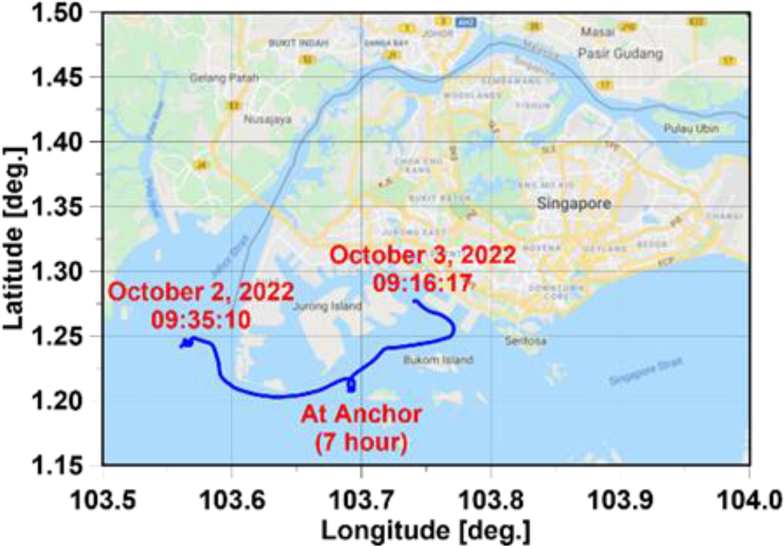
The AIS data was collected through an open-source platform from the automatic identification system at the National University of Singapore. In this study, the data from October 2022 was selected as the study data. This dataset contains substantial information, including more than 7,371,647 data lines relating to more than 22,000 ships and marine vehicles. The AIS data is filtered based on the Maritime Mobile Service Identity (MMSI) number, so that data should be of good quality, with few errors or little missing data. For the purpose of this study, data associated with the MMSI number 636017059 was chosen. The principal dimensions of the ship are described in Table 1.
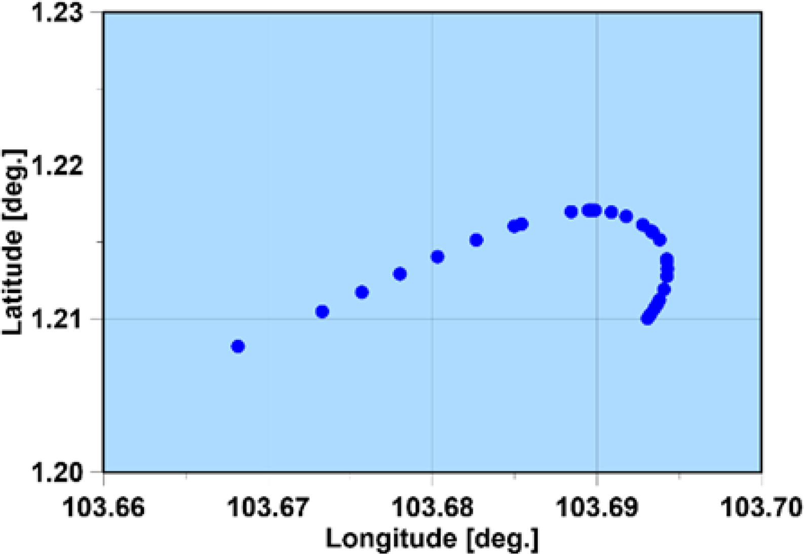
Fig. 1 shows the actual trajectory of the Silverway ship. To facilitate the estimation of the hydrodynamic coefficients, a small trajectory segment has been selected. This trajectory was a segment where the ship turned in a circle to starboard before reaching the mooring area. The selected trajectory segment is shown in Fig. 2.
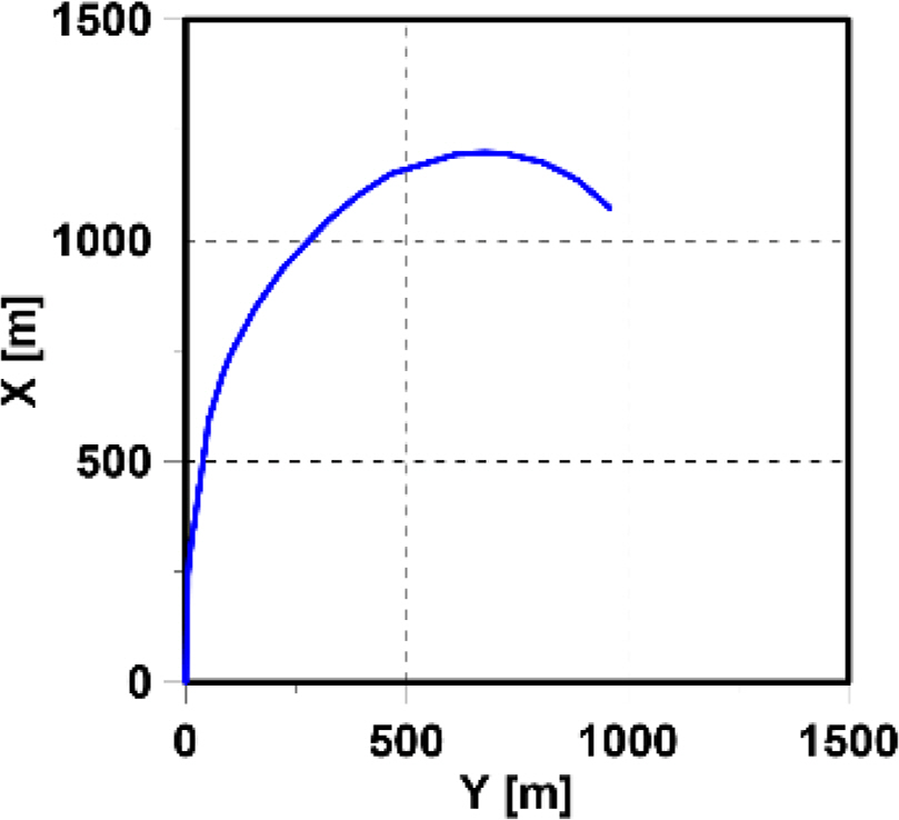
AIS data includes data such as longitude, latitude, speed over ground (SOG), rate of turn (ROT), course over ground (COG) and heading angle (HDG). These are the data needed to initialize the training data. First, the conversion process involved converting the geographic coordinates of longitude and latitude in the World Geodetic 1984 (WGS84) system into the X and Y coordinates in the Universal Transverse Mercator (UTM) coordinate system. Second, Mou et al. (2013) calculated the rudder angle using AIS data. The rudder angle was calculated from ROT and HDG using Nomoto’s model and Ridge regression method. The Nomoto’s model can be expressed as Eq. (1).
where ṙ is the yaw angular acceleration, and r is the yaw rate. δ is the rudder angle. T is the time constant, and K is the proportionality constant.
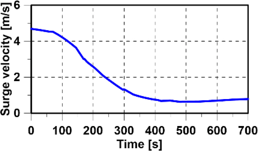
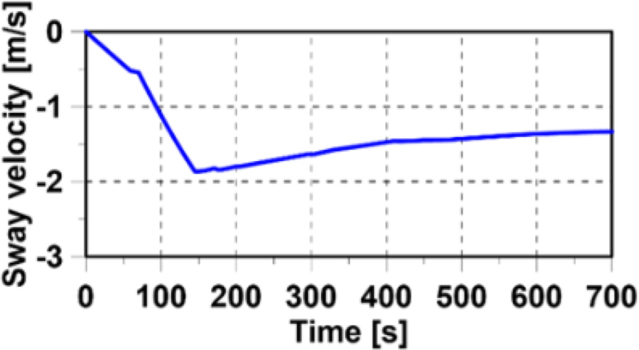
Finally, Inazu et al. (2020) described the velocity and direction vectors of the ship. The surge and sway velocities are determined by SOG, COG and HDG as expressed in Eq. (2). The results of X and Y coordinates, rudder angle, surge velocity and sway velocity are shown in Figs. 3,–6, respectively.
The data measurement time in AIS data ranges from a few seconds to several tens of seconds because it depends on the speed and course alteration of a ship. Therefore, the linear interpolation method was applied to interpolate the missing points based on the time variable. The interval time selected for interpolation is 1 second to synchronize with the interval time in the hydrodynamic coefficient estimation algorithm and ship maneuvering simulation.
3. Methodology
3.1 Equation of Ship Maneuvering Motion
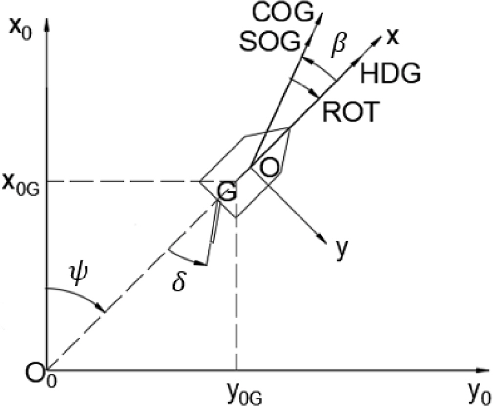
In ship maneuvering, the coordinate system fixed to the earth and the fixed coordinate system of the hull are applied. The Earth-fixed coordinate system (O0x0y0) has the origin as the position of the center of gravity of a ship at time t0. The body-fixed coordinate system (Oxy) is assumed to be at the midship. The x0-axis is set in the direction of the initial course of the ship, the y0-axis points to the left, and the z0-axis points up. While the x-axis points toward the bow, the y-axis points to starboard, and the z-axis points downwards. The angles between the directions of velocity V and the x-axis are defined as the drift angle β. The angles between the directions of the x0-axis and x-axis are defined as the heading angles ψ. The coordinate systems in ship maneuvering are shown in Fig. 7.
Abkowitz maneuver model in 3DOF is considered to describe the forces and moment acting on the ship. These motions are expressed as non-dimensional in Eq. (3).
where the superscript represents non-dimensional variables; m′ is the ship mass; x′G is the longitudinal center of gravity in the body-fixed coordinate system; I′z is the inertia moment about the z-axis; u̇′, v̇′ and ṙ′ are the accelerations in the x-axis, y-axis, and z-axis, respectively; X′u̇, Y′v̇, Y′ṙ, N′V̇, and N′ṙ are the acceleration derivatives; f′1 and f′2 are forces in the x-axis and y-axis, respectively, and f′3 is the moment about the z-axis. These forces and moment are displayed as functions of the kinematic parameters and rudder angle by applying the Taylor-series expansion extended to a third-order function, as expressed in Eq. (4).
f ′ 1 = X ′ u u ′ + X ′ u u u ′ 2 + X ′ u u u u ′ 3 X ′ v v v ′ 2 + X ′ δ δ δ 2 + X ′ u δ δ u ′ δ + X ′ r v r ′ v ′ + X ′ v δ v ′ δ + X ′ v δ u v ′ δ u ′ f ′ 2 = Y ′ v v ′ + Y ′ r r ′ + Y ′ v v v v ′ 3 + Y ′ v v r v ′ 2 r ′ + Y ′ v u v ′ u ′ + Y ′ r u r ′ u ′ + Y ′ δ δ + Y ′ δ δ δ δ 3 + Y ′ u δ u ′ δ + Y ′ u u δ u ′ 2 δ + Y ′ v δ δ v ′ δ 2 + Y ′ v v δ v ′ 2 δ + Y ′ 0 + Y ′ 0 u u ′ + Y ′ 0 u u u ′ 2 f ′ 3 = N ′ v v ′ + N ′ r r ′ + N ′ v v v v ′ 3 + N ′ v v r v ′ 2 r ′ + N ′ v u v ′ u ′ + N ′ r u r ′ u ′ + N ′ δ δ + N ′ δ δ δ δ 3 + N ′ u δ u ′ δ + N ′ u u δ u ′ 2 δ + N ′ v δ δ δ v ′ δ 2 + N ′ v v δ v ′ 2 δ + N ′ 0 + N ′ 0 u u ′ + N ′ 0 u u u ′ 2
(4)
3.2 Reconstruction of Ship Maneuvering Model
For the purpose of parameter identification, Eq. (3) is rewritten as Eq. (5). In Eq. (5),
S = ( I z ' - N r ˙ ' ) ( m ′ - Y v ˙ ' ) - ( m ′ x G ' - Y r ˙ ' ) ( m ′ x G ' - N v ˙ ' )
By combining Eqs. (5) and (6), the symbol vectors can be expressed as Eq. (7). Symbol vectors include variable vectors of X, Y, and Z, and coefficient vectors of A, B, and C. Variable vectors X, Y, and Z are the non-dimensional hydrodynamic derivatives of surge, sway, and yaw motions, respectively. The coefficient and variable vectors are expressed as Eq. (8) and Eq. (9), respectively.
X = [ u ( k ) U ( k ) , u 2 ( k ) , u 3 ( k ) / U ( k ) , v 2 ( k ) , r 2 ( k ) L 2 , Δ δ 2 ( k ) U 2 ( k ) , Δ u ( k ) Δ δ 2 ( k ) U ( k ) , Δ v ( k ) Δ r ( k ) L , Δ v ( k ) Δ δ ( k ) U ( k ) , Δ v ( k ) Δ δ ( k ) Δ u ( k ) ] 10 × 1 T Y = N = [ Δ v ( k ) U ( k ) , Δ r ( k ) U ( k ) L , Δ v 3 ( k ) / U ( k ) , Δ v 2 ( k ) Δ r ( k ) L / U ( k ) , Δ v ( k ) Δ u ( k ) , Δ r ( k ) Δ u ( k ) , Δ δ ( k ) U 2 ( k ) , Δ δ 3 ( k ) U 2 ( k ) , Δ u ( k ) Δ δ ( k ) U ( k ) , Δ u 2 ( k ) Δ δ ( k ) , Δ v ( k ) Δ δ 2 ( k ) U ( k ) , Δ v 2 ( k ) Δ δ ( k ) , U 2 ( k ) , Δ u ( k ) U ( k ) , Δ u 2 ( k ) ] 15 × 1 T
(9)
For example, the longitudinal hydrodynamic coefficient X′u is defined using Eq. (10). This equation was also applied to determine the other hydrodynamic coefficients of the surge equation.
The same method is used to estimate the hydrodynamic coefficients of sway and yaw equations. A series of equations and matrices need to be solved to determine the hydrodynamic coefficients of sway and yaw. For example, the hydrodynamic coefficients Y′v and N′v are obtained by solving Eq. (11). The other hydrodynamic coefficients of the sway and yaw equation are also obtained similarly.
The five acceleration derivatives
X u ˙ ′ Y v ˙ ′ Y r ˙ ′ N v ˙ ′ N r ˙ ′ X u ˙ ′ = − 0.001135 Y v ˙ ′ = 0.014508 Y r ˙ ′ = − 0.001209 N v ˙ ′ = − 0.000588 N r ′ = − 0.000564
3.3 Support Vector Regression
SVR has a general approximation function for a multi-input/single-output (MISO) system:
where f(xi) is the scalar output; w is the weight matrix; b is the bias; xi is the input vector; ℝn is the n-dimensional feature space, and Φ(xi) is a linear or non-linear and refers to the high-dimensional feature space ℝN (N >> M). In SVR, the regression issue is viewed as an optimization problem in the primal formula subject to an objective function and constraint formula, as expressed in Eqs. (13) and (14), respectively.
where C is called the regularization parameter. This parameter is always positive, which is designed to control the trade-off between empirical error and model complexity. ξ and ξ* are the slack variables. It defines the upper limit of regression errors until the constraints are still satisfied. In Eq. (14)y and ∊ are the desired output and an insensitivity factor, respectively. The loss quantification is determined by the distance between the boundary ε and the observed value y shown in Eq. (15).
By using the Karush-Kuhn-Tucker (KKT) theorem and Lagrange dual formulation, Lagrange multiples αn and
α n *
The optimal hyperplane can be obtained as Eq. (18) to predict new values depending only on the support vectors:
The w and b parameters can be described entirely as a linear combination using a linear kernel:
where the dash on top of Eq. (20) and N refer to the mean value and the total number of support vectors.
4. Result
4.1 Algorithm Validation
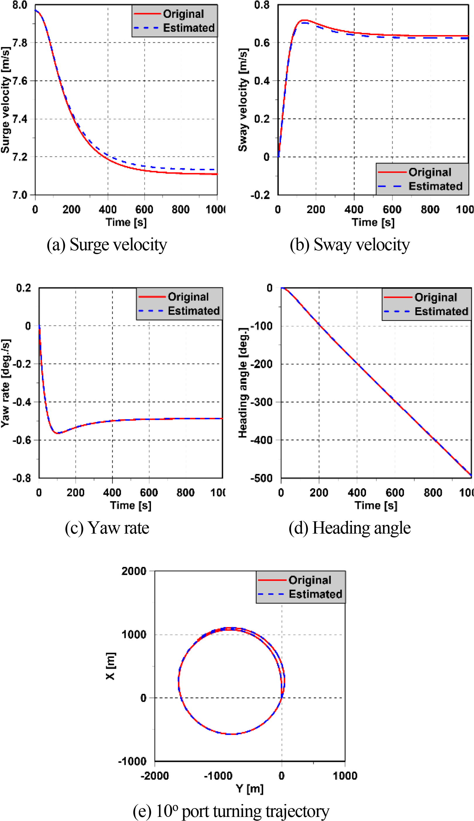
Validating the accuracy and performance of the SVR algorithm is done by estimating the hydrodynamic coefficients of the Mariner class vessel. Fossen (1994) described these coefficients in the Abkowitz model. These coefficients were applied to simulate the turning circle test at a rudder angle of 10°. The simulation results were used as training data for the SVR model. Luo and Zou (2009) and Luo (2016) referred to the multicollinearity and parameter drift phenomenon. The hydrodynamic coefficients may be inaccurate or worse, even if the simulation results match well with the target results. A proposed solution to reduce these two phenomena is to add Gaussian noise to the training data. Applying the SVR algorithm and Gaussian noise, the hydrodynamic coefficients are estimated and compared with the original hydrodynamic coefficients. The ship parameters and simulated conditions are described in Table 2. The results of hydrodynamic coefficients are shown in Tables 3,–5.
The turning circle test was simulated from the estimated hydrodynamic coefficients and compared with the original simulation results in Fig. 8. The deviations between the estimated hydrodynamic coefficients and the original hydrodynamic coefficients are very low. Therefore, they matched the training data and the regression model well.
In addition, the SVR algorithm is well-validated. In addition, the SVR algorithm is well-validated. Of the 40 hydrodynamic coefficients for the surge, sway and yaw equation, the
Y v δ δ ′ Y 0 u u ′ N v v v ′ N v v δ ′ N 0 u ′
4.2 Hydrodynamic Coefficients of Silverway Ship in AIS Data
After validating the SVR algorithm, the hydrodynamic coefficients of the Silverway ship in AIS data are estimated. In this case, Gaussian noise is not considered because Luo (2016) suggested that this method is unsuitable for AIS data. Ship parameters and simulated conditions are shown in Table 6. This simulation condition is established based on the calculation results of the rudder angle from the AIS data. The time required for the rudder angle to change from 0° to approximately 10° was approximately 163 seconds. Therefore, the maximum rudder angle derivative is defined as 0.06°/s.
The result of the hydrodynamic coefficients for the surge, sway and yaw equations are shown in Tables 7 and 8. AIS data typically represents real-world ship movements and provides a reference for evaluating the accuracy and validity of the simulation results. When comparing the simulation results with AIS data, the goal was that the simulated trajectories closely match the observed ship movements. Therefore, the turning circle test was simulated from estimated hydrodynamic coefficients and compared with the AIS data in Fig. 9. Generally, the simulation results from the estimated hydrodynamic coefficients were in good agreement with the AIS data. Therefore, the estimated hydrodynamic coefficients are reliable. Moreover, the SVR algorithm is also successfully applied to AIS data.
5. Conclusions
In conclusion, this study aimed to estimate the hydrodynamic coefficients of Silverway ship in AIS data using the Linear SVR model. The study used the simulation results of the maneuvers of the Mariner class vessel to validate the accuracy and suitability of the estimated hydrodynamic coefficients.
First, the collection and conversion of AIS data into a usable form have been successfully accomplished for the purpose of hydrodynamic coefficient estimation. The transformed AIS data provides valuable information on vessel identification, position, speed, and course, which is essential for further analysis and modeling in ship maneuvering studies.
Secondly, the SVR algorithm is validated by estimating hydrodynamic coefficients using the Mariner class vessel simulation results. When applying the method of adding Gaussian noise to reduce the multicollinearity and parameter drift phenomena, the estimated hydrodynamic coefficients matched well with the original coefficients. This demonstrated the accuracy and efficiency of the SVR algorithm. In addition, it confirmed the suitability of adding Gaussian noise to the results of ship maneuvering simulations.
Finally, the hydrodynamic coefficients of Silverway ship in AIS data were estimated using the validated SVR algorithm. The results show that the estimated hydrodynamic coefficients and the simulated movements are in good agreement with the AIS data. Therefore, it is possible to apply the SVR model to AIS data.