Validation of OpenDrift-Based Drifter Trajectory Prediction Technique for Maritime Search and Rescue
Article information

Abstract
Due to a recent increase in maritime activities in South Korea, the frequency of maritime distress is escalating and poses a significant threat to lives and property. The aim of this study was to validate a drift trajectory prediction technique to help mitigate the damages caused by maritime distress incidents. In this study, OpenDrift was verified using satellite drifter data from the Korea Hydrographic and Oceanographic Agency. OpenDrift is a Monte-Carlo-based Lagrangian trajectory modeling framework that allows for considering leeway, an important factor in predicting the movement of floating marine objects. The simulation results showed no significant differences in the performance of drift trajectory prediction when considering leeway using four evaluation methods (normalized cumulative Lagrangian separation, root mean squared error, mean absolute error, and Euclidean distance). However, leeway improved the performance in an analysis of location prediction conformance for maritime search and rescue operations. Therefore, the findings of this study suggest that it is important to consider leeway in drift trajectory prediction for effective maritime search and rescue operations. The results could help with future research on drift trajectory prediction of various floating objects, including marine debris, satellite drifters, and sea ice.
1. Introduction
Marine leisure activities have recently increased, resulting in an increase in maritime distress, which poses a threat to lives and property. The Korea Coast Guard (KCG) provides statistics on accidents that occur in different maritime police jurisdictions. From 2017 to 2021, maritime distress accidents in South Korea have been continuously increasing, and in about 31% of maritime accidents, it has been difficult to locate missing people. Accidents caused by a loss of vessel power, capsizing, sinking, and grounding account for about 28.3% of all accidents, while about 29.5% are caused by flooding, fire, and collision, which have various possibilities depending on the response after the accident. About 67.5% of all accidents occur in good weather conditions, and the remaining 32.5% occur in poor weather conditions such as storm warnings, rough weather, and low visibility. Fishing vessels accounted for the majority of vessel types and were involved in 78.9% of all accidents (KCG, 2022b).
According to Article 2 of the “Act on the Search and Rescue in Waters”, maritime distress is defined as situations where human life, physical safety, or the safety of vessels are at risk on the water. Vessels, lifeboats, people, and other objects involved in maritime distress tend to drift due to various external forces such as wind, tidal currents, ocean currents, and waves. As time passes, they move increasingly further away from the point of an accident. This characteristic leads to a high mortality rate and makes search and rescue (SAR) operations difficult, incurring significant costs. Therefore, in order to reduce casualties in events of maritime distress, it is important to quickly and accurately estimate the location of distressed objects and determine the search area (Kang, 1998).
To estimate the location of drifting objects, the total vector is calculated while considering various oceanic external forces from the starting point of the distress occurrence or the last reported accident location, which allows for an estimation of the hourly position of drifting objects (Yun et al., 2001). The initial location and time of the occurrence of maritime distress depend on reports from individuals or entities involved in the accident or surrounding vessels, so they contain some margin of error. Depending on the navigational device used for the initial position measurement, the error may range from meters to hundreds of meters, and the time of distress may vary from minutes to several hours (Lee et al., 1999). According to Tipton et al. (2022), the major factors determining the survival rate of individuals immersed in water include water temperature, accident area, age of the survivor, clothing, and whether a life jacket was worn. Generally, the survival rate remains relatively high at around 80% for about 4–5 h after the onset of drifting. However, survival rates drastically drop to about 40% after this period, and by 14 h, the survival rate reaches 0%.
In South Korea, a law was enacted in 1961 for the handling of rescue operations involving distressed vessels and individuals and the preservation of life and property. Legal amendments were made in 1994 and 1996 to facilitate South Korea's accession to and compliance with the International SAR Convention. In 2012, the law was revised to reflect changes due to the increase in marine leisure. The law was renamed the “Act on the Search and Rescue in Waters,” which stipulates the authority of the chief of rescue and the duty of the captain and crew of distressed vessels to participate in rescue operations. In 2021, an amendment was made to promote the participation of private maritime rescue team members. Now, the act is the law that protects the lives and property of citizens in the event of maritime distress and supports private maritime rescue activities (KCG, 2022a).
The Korea Hydrographic and Oceanographic Agency (KHOA) has established and operates an ocean current prediction system to provide consistent support for SAR operations by relevant agencies in the event of maritime distress. The KHOA is improving techniques to predict drift trajectories for maritime SAR activities by conducting drift prediction experiments using satellite drifters to improve accuracy (KHOA, 2022). Previous research predicted the trajectory of satellite drifters using machine learning and the features of ocean currents and wind, such as their strength and direction (Lee et al., 2017; Kim and Kim., 2018; Seo, 2021; Ha et al., 2022). Lee et al. (2017) used machine learning techniques to improve the “Modelo Hidrodinamico” (MOHID) numerical model and develop a model for predicting the trajectories of satellite drifters. Kim and Kim (2018) proposed a data correction model using recurrent neural networks and autoencoders to address possible errors or missing data observed using satellite drifters. Seo (2021) conducted a study on a new feature generation method for predicting the trajectories of satellite drifters using the support vector machine (SVM), k-nearest neighbor (k-NN), and random forest methods based on observational data from satellite drifters. Ha et al. (2022) compared and analyzed a particle-tracking model based on a numerical ocean model with a model based on observation data.
According to the International Maritime Organization (IMO), SAR refers to the operations conducted using aircraft, vessels, submarines, and special equipment to find distressed persons. The IMO adopted the International Convention on Maritime SAR in 1979, establishing an international SAR system. There are over 80 SAR Convention countries, including the United States, Japan, China, Russia, and Korea, and these countries have a duty to establish SAR organizations and support the SAR operations of neighboring countries when necessary (Park et al., 1989).
In 1999, the IMO and the International Civil Aviation Organization (ICAO) jointly developed the International Aeronautical and Maritime SAR manual (IAMSAR) for use as national SAR guidelines in all SAR Convention signatory countries. The IAMSAR manual reflects the reality of maritime distress, which is highly uncertain, and supports the decision-making of SAR personnel. However, given the nature of the manual, all data must be manually entered to derive results, which makes rapid response difficult in the event of maritime distress. As a result, leading maritime nations like the United States and Canada are investing heavily in field experiments for distressed objects and the development of ocean current measurement buoys to accurately track the location of distressed vessels (Yun, 2005). They have also developed and are operating SAR planning programs like the SAR optimal planning system (SAROPS) and SARMAP (Fig. 1).
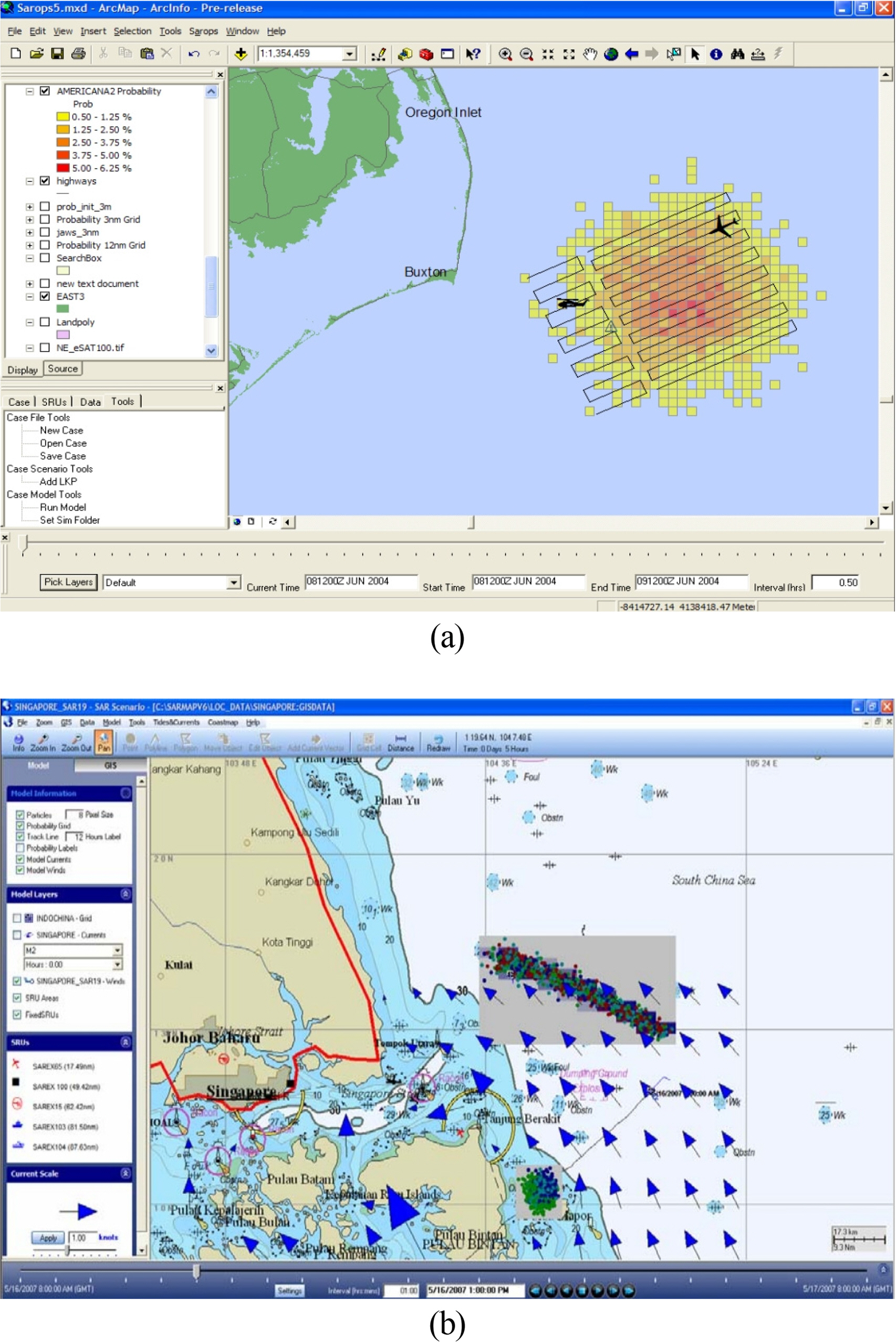
Search and rescue plan generation program operated internationally: (a) SAROPS (U.S. Coast Guard); (b) SARMAP (RPS Group)
Leading maritime nations have implemented an integrated system that incorporates the prediction of a drifter's locations to calculate the probability of containment (POC), probability of detection (POD), and ultimately the probability of success (POS), which are utilized in search planning. In South Korea, the KCG is the agency responsible for maritime SAR and utilizes the Ocean Current Prediction System developed by the KHOA for estimating the locations of drifters. The ocean current prediction system analyzes marine meteorological data such as ocean currents and winds to predict the trajectory of drifters and track the trajectories of vessels or missing individuals. Currently, there is no equivalent search evaluation system to that in other countries (Yun, 2020).
According to Breivik and Allen (2008), there is a need for probabilistic representation to calculate the uncertain movement of drifting maritime objects. Instead of predicting the exact trajectory of the object, they found the area where the drifting object is most likely to be located by altering various parameters that influence the movement of the object using the Monte Carlo technique and calculating a search area. Given that South Korea has a complex coastline and significant differences in the local characteristics of the ocean, continued efforts are being made to develop high-resolution numerical models and carry out various verifications to simulate ocean currents accurately. However, due to the high degree of uncertainty in the movement of maritime drifting objects, it is essential to consider unpredictable factors related to environmental forces in predictions. But most studies conducted in South Korea have been limited to evaluating the accuracy of models by analyzing the performance of ocean numerical models and machine learning-based prediction of maritime drifting object trajectories, making it difficult to consider the uncertain factors in the marine environment. Furthermore, although there have been field studies to derive the leeway parameters, there have not been many experiments on predicting the probabilistic trajectory of drifting objects using them.
Therefore, in this study, simulations were performed using OpenDrift, which allows Monte-Carlo-based random particle trajectory predictions to consider uncertain factors in drift movement represented by leeway. The aim of this study was to confirm the performance of OpenDrift simulations through an evaluation method proposed in previous research. An analysis method and prediction results are presented for evaluating the applicability to maritime SAR to help reduce the damage from maritime distress.
2. Drifter Trajectory Prediction
2.1 Leeway
Among the external forces acting on maritime objects, the ocean current and wind are considered the most significant. Leeway refers to the amount of movement of a drifting object caused by the wind acting on the exposed surface of the drifter and is typically calculated using information observed from maritime drifter experiments regarding ocean current, wind, and drifter location (Yun et al., 2001). The way of expressing the leeway formula varies slightly depending on the researcher. Notably, early research such as that by Hufford and Broida (1974) represented leeway as the leeway speed and divergence angle, while Allen and Plourde (1999) represented leeway as a downwind leeway component (DWL), a component parallel to the wind, and a crosswind leeway component (CWL) that is perpendicular to the wind. CWL is a positive (+) value when the direction of the leeway is to the right and a negative (-) value when it is to the left (Fig. 2).

Relationship between the leeway speed, downwind, and crosswind components of leeway (Allen and Plourde, 1999)
Several SAR models have been developed internationally to reflect the effects of leeway (Fig. 3). The geographic display operations computer automated manual method (GDOC AMM) is a computerized program that uses the method in the national SAR manual (NATSAR) issued by the United States Coast Guard (USCG). It always applies 100% ocean surface current when calculating drift distance and determines the search area based on leeway speed and divergence angle. The computer-aided search planning (CASP) model assumes that basic variables such as time, location, current, and wind have a probability distribution through Monte Carlo simulation. It applies an uncertainty coefficient of 0.33 to the leeway rate to repeatedly calculate the drift location. The AP98 model developed by Allen and Plourde uses the slope and y-intercept of the leeway equation. The location of a drifting object is probabilistically calculated by randomly altering the slope and y-intercept, assuming a normal distribution with a standard deviation of Sy/x (Allen and Plourde, 1999).
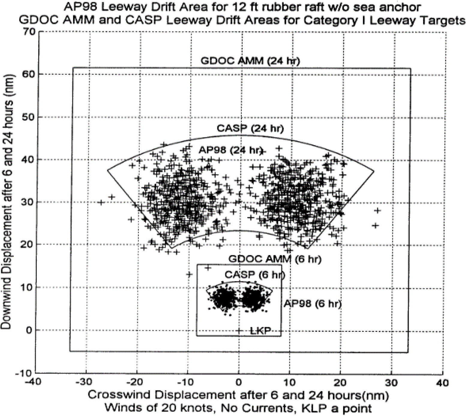
The leeway drift area of a leeway distribution model (Allen and Plourde, 1999)
2.2 Drifter
The KHOA is conducting experiments using satellite-tracked drifters to improve the accuracy of ocean current predictions. They provide data through the “Badanuri Marine Information Service.” Since 2016, the surface velocity program (SVP) has been providing data, and since 2019, data from SVP and surface satellite-tracked drifters have been available. The SVP uses a drogue installed below a buoy with a diameter of less than 40 cm (Fig. 4), while the surface satellite-tracked drifters are small cylindrical buoys with a diameter of 10 cm and a length of 30 cm.
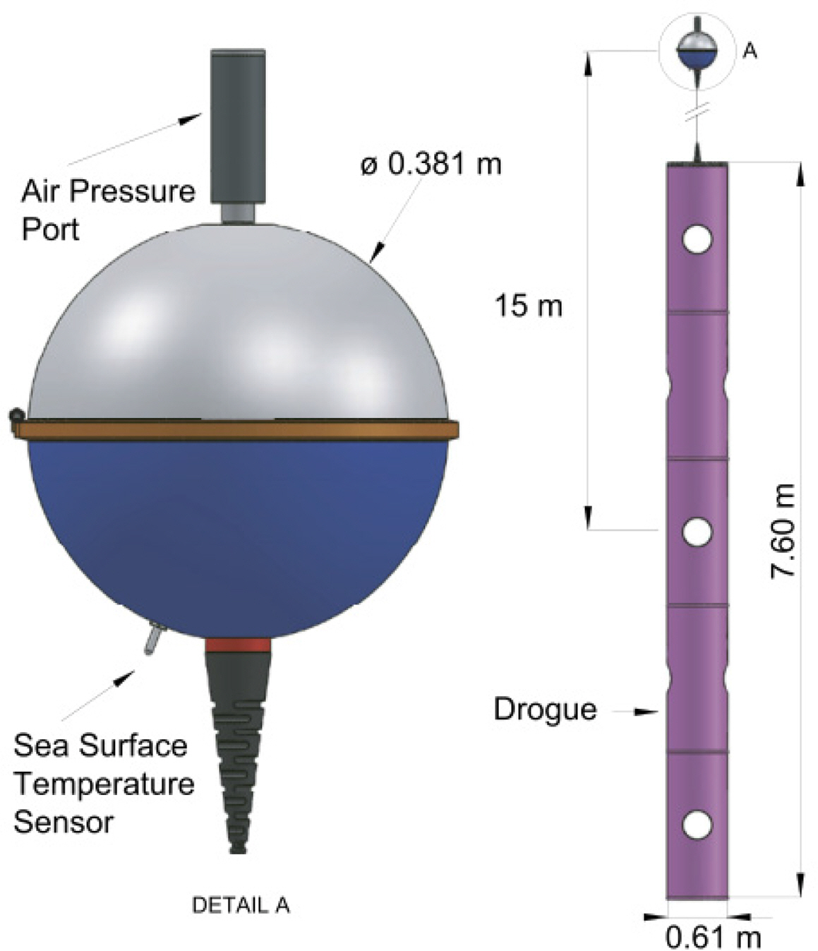
Specifications of KHOA SVP (Centurioni et al., 2017)
The leeway effect caused by wind is important in predicting the movement of maritime drifters. However, the surface satellite-tracked drifters are not suitable for considering the leeway effect due to their small exposed area on the water surface. The SVP is an international research program that is widely used in oceanography, climatology, weather forecasting, and other marine-related research fields. It focuses on measuring speeds at the ocean surface and significantly contributes to enhancing understanding of various marine environmental variables such as ocean circulation, sea surface temperature, and wind patterns (Lumpkin and Pazos, 2007). In this study, data from the KHOA SVP were used to consider the leeway effect on satellite-tracked drifters.
Cho et al. (2014) conducted field experiments on buoy C, which is a cylindrical buoy with a diameter of 50 cm and a height of 30 cm and has a drogue installed. Their leeway parameters for buoy C are provided in Table 1. Buoy C is similar to the KHOA SVP, and in this study, the values from buoy C were used as the leeway parameters for the drifters. Experiments were conducted using the location data of an SVP satellite-tracked drifter (ID: 300434063234840), which was deployed in the Jeju Strait in July 2019. The data were acquired from the KHOA's Badanuri Marine Information Service.
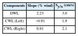
Leeway coefficients of buoy C (Cho et al., 2014)
2.3 OpenDrift
OpenDrift is a software package developed by the Norwegian Meteorological Institute (NMI) for simulating the trajectories and endpoints of maritime drifters. It is implemented as a Python-based open-source framework for Lagrangian particle modeling. OpenDrift is designed to be fast and easy to use and supports various operating systems such as Linux, Mac, and Windows. It offers the advantage of providing different libraries, allowing researchers to choose modules that suit their specific purposes. While the detailed workflow may vary depending on the selected modules, the general process follows the framework illustrated in Fig. 5.
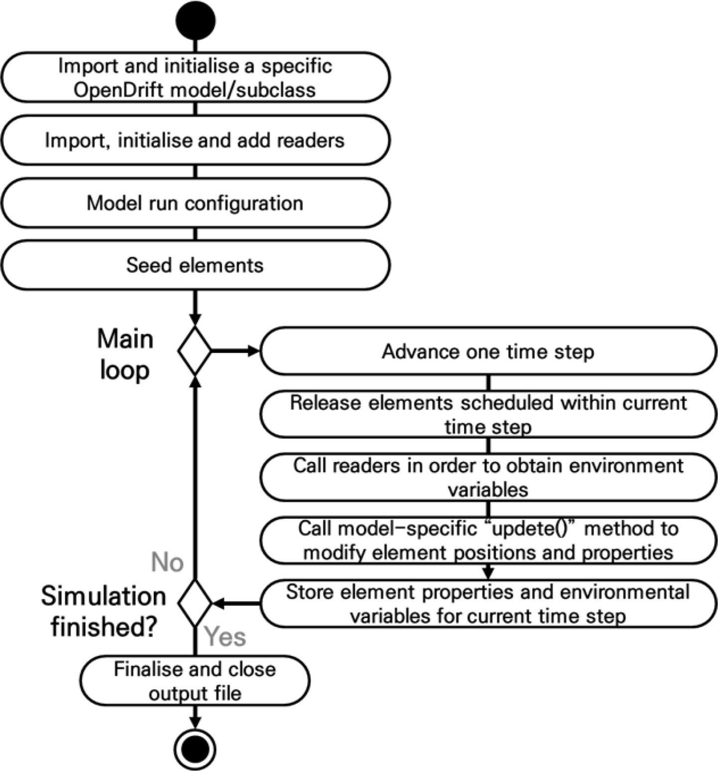
Flowchart of an OpenDrift simulation (Dagestad et al., 2018)
OpenDrift’s key components are the reader and basemodel classes in the module execution. The reader class reads external forcing data such as wind, wave, and ocean current data from numerical model data following the climate and forecast (CF) naming convention. It inputs the time series values of each grid into the OpenDrift module. The basemodel class provides common functionalities that are applicable to all drift prediction models for calculating the new positions of each particle based on the module execution (Dagestad et al., 2018).
Among the libraries in OpenDrift, the oceandrift module is the most basic module for predicting particle movement based on numerical models of ocean currents. Factors affecting particle movement include advection, wind drag, Stokes drift, turbulent mixing, vertical advection, and machine learning. The module allows for consideration of horizontal diffusion and the influence of wind speed through the wind drift factor. The leeway module predicts particle movement based on numerical models of ocean currents and winds. It incorporates leeway parameters using the AP98 model representation, as specified by Allen and Plourde (1999) and Breivik and Allen (2008), and there are 85 types of drifters in total. The leeway parameters are internally embedded and are used when calculating the linear regression relationship between leeway speed and wind speed using the least square method. The calculations are done using Eqs. (1)–(3).
In these equations, Uwind and Vwind represent the magnitude of the x-direction and y-direction winds from the input numerical model data. Slope and Offset refer to the slope and y-intercept of the leeway equation, respectively. ϵn is a value obtained by applying a random number from a normal distribution to the leeway’s standard deviation, while an and bn are values that reflect randomness in the Slope and Offset. Each particle in OpenDrift is determined to move to the next location based on the vector sum of the calculated ocean current and leeway (Dagestad et al., 2018).
2.4 Simulation Setup
To run OpenDrift, numerical model data for oceanic forcing are required. The oceandrift module requires numerical models of ocean currents, while the leeway module requires numerical models of both ocean currents and winds. In this study, the hybrid coordinate ocean model (HYCOM) and korea local analysis and prediction system (KLAPS) were used for numerical model data for oceanic forcing. Detailed information about the numerical models is provided in Table 2.

Numerical model information used as input data for OpenDrift
In a previous study, simulations were performed to evaluate the performance of trajectory prediction using forecast data (Liu and Weisberg, 2011). In these simulations, initial locations were released at regular time intervals along the drifter trajectories. The findings confirmed that the release interval time had minimal impact on the skill score. Additionally, if the simulation time is too short, the cumulative distance of the observations can be small, leading to increased uncertainty. Therefore, the simulation time was set to 72 h.
Based on the study by Liu and Weisberg (2011), particles were released at regular intervals along drifter trajectories to perform simulations. However, compared to the previous study, the simulation period in this research was very short, ranging from July 25, 2019, 0:00, to July 28, 2019, 23:00 (KST). If the release interval time for initializing the locations is set too long, the experiment data would be limited, making it difficult to ensure statistical reliability. Therefore, before conducting the experiments, a preliminary experiment was carried out by gradually increasing the interval for initializing the locations from 1 hour to 24 h with intervals of 1 h.
The aim of the preliminary experiment was to examine whether there would be significant changes in the skill score with different intervals for initializing the locations. The results of the preliminary experiment showed that even with a release interval time shorter than 24 h, there were no significant changes in the skill score (Fig. 6). Based on these preliminary results, the interval for releasing the initial locations was set to 1 hour to enhance the statistical reliability of the simulation results, resulting in a total of 96 cases of simulation data.

Sensitivity of the skill scores to the drifter release interval
To understand the impact of the leeway on the trajectory prediction results, both the leeway module and the oceandrift module were applied under the same conditions. The particle stranding option was set to “off” in both the leeway module and the oceandrift module, while the remaining parameters such as the wind drift factor and current drift factor were set to their default values. Based on previous studies, each simulation was set to run for 72 h. In order to obtain statistically significant results, 1000 particles were randomly seeded within a 1-km radius, which followed a normal distribution (Fig. 7).
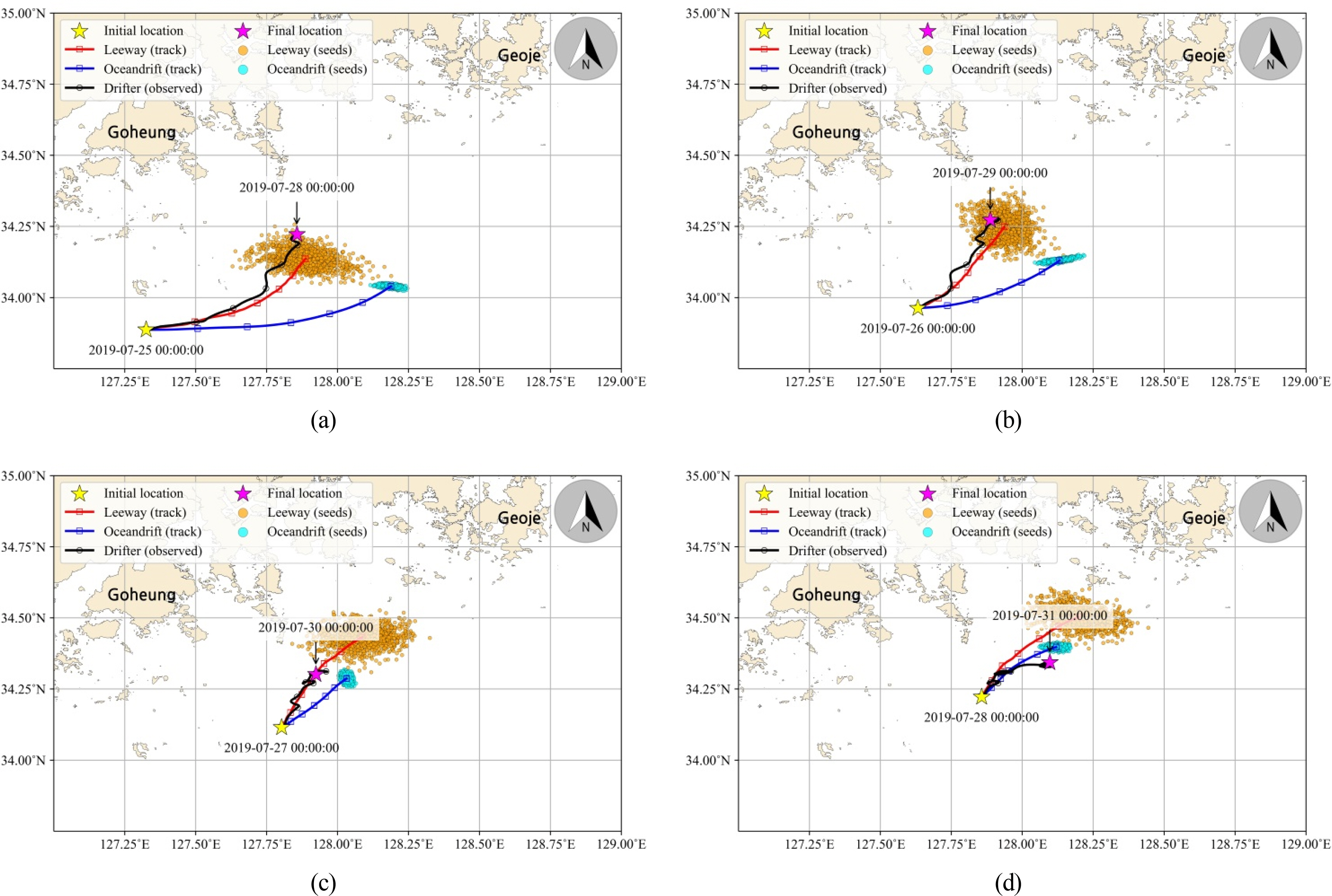
Simulation results of OpenDrift during 72 h. The black solid line represents a satellite drifter (observed). The blue solid line represents the oceandrift module’s results showing the average particle location at each time step. The red solid line represents the leeway module’s results showing the average particle location at each time step. The light blue circle represents the particle distribution after 72 h of oceandrift module operation. The orange circle represents the particle distribution after 72 h of leeway module execution. Simulation results of OpenDrift at 0 h KST on (a) July 25th, (b) July 26th, (c) July 27th, and (d) July 28th.
3. Validation of Simulation Results
3.1 Comparison Method of Predicted Drifter Trajectories
To validate the drifters trajectory prediction performance of OpenDrift, various evaluation methods were applied: the normalized cumulative Lagrangian separation (NCLS) evaluation proposed by Liu and Weisberg (2011), the root mean squared error (RMSE) evaluation considered by Dominicis et al. (2013), and the mean absolute error (MAE) and Euclidean distance (Euclid) evaluations used by Nam and Kim (2018). The NCLS calculates the separation distance based on the difference between observations and numerical solutions, and a skill score close to 1 indicates a perfect simulation (Fig. 8). The RMSE quantitatively represents the difference between observations and numerical solutions, and the larger the deviations, the higher the values of the RMSE are. While it provides a numerical representation of the errors, it is challenging to interpret the extent of the errors (Kim and Yoon, 2011). The MAE represents the mean error value quantitatively, and the Euclidean distance represents the average distance between particles. Lower values in both evaluations indicate better prediction performance (Nam and Kim, 2018).
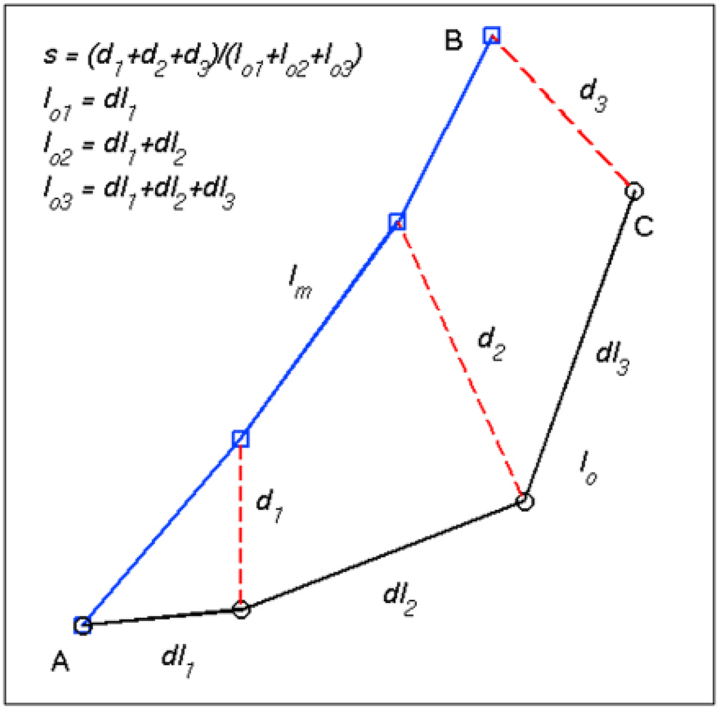
A diagram illustrating the calculation method of NCLS (Liu and Weisberg, 2011)
In Eqs. (4)–(5), di represents the separation distance between observations and the simulation result, loi represents the cumulative sum of the observed displacement distances, and N represents the total number of data points. s denotes the normalized cumulative separation, and n is a dimensionless value representing the allowed threshold. A smaller value of n indicates a stricter criterion for the simulation. In this study, a value of n = 1 was adopted, which was used by Nam and Kim (2018) and Ha et al. (2022).
In Eq. (6)d represents the separation distance between the i-th model position (Si) and the i-th observed position (Oi), while N denotes the total number of observations.
In Eqs. (7)–(8), Lat(M) and Lon(M) represent the latitude and longitude of the predicted model, respectively, while Lat(O) and Lon(O) represent the latitude and longitude of the observations. N represents the total number of observations.
3.2 Method for Evaluating Applicability in Maritime SAR
SAROPS, SARMAP, and other SAR support programs utilize random particle-based Monte Carlo simulations to account for the uncertainties in drifter movement. Based on the simulation results, search areas are established. Therefore, for an accurate simulation, it is necessary for the actual drifters to be located within the predicted area. To assess the effectiveness of the OpenDrift results for maritime SAR operations, the presence or absence of actual drifters within the predicted area was determined at each specific time. This concept is defined as location prediction conformance (LPC) in this study.
In Eq. (9)C represents whether an actual drifter is included within the predicted area. Its value is 1 if the drifter is within the area, as shown in Fig. 9(a), while it is 0 if the drifter is outside the area, as in Fig. 9(b). N in Eq. (10) is the total number of data and represents the probability of the drifter’s location over the entire period, which is assessed by determining the presence at each time from the simulation results. The criterion for the predicted area is based on representing the Monte-Carlo-based simulation results of Breivik and Allen (2008) as polygonal areas (convex hulls) and it is set as a polygonal area connecting the outermost area of the particles simulated by OpenDrift.
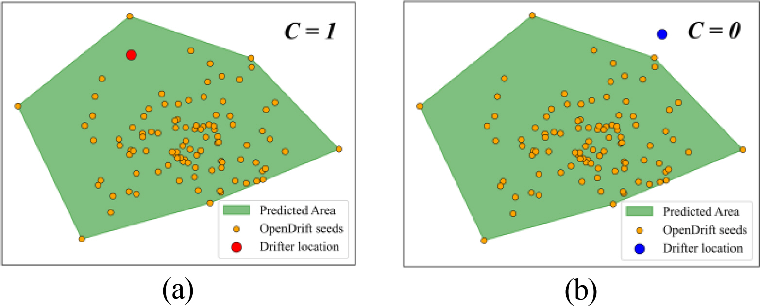
Method for determining the presence of observed drifters within a predicted model area. (a) Satellite drifter included within the prediction area (red circle) and (b) Satellite drifter not included within the prediction area (blue circle)
4. Analysis Results
4.1 Assessment of Predictive Performance Over Simulation Elapsed Time
The results of the performance analysis with different simulation durations are shown in Fig. 10. The RMSE, MAE, and Euclid scores tended to increase as the simulation time elapsed, while the NCLS score tended to decrease. Lower RMSE, MAE, and Euclid values and higher NCLS values indicate higher prediction accuracy, which means that the overall prediction accuracy decreases with the passage of simulation time (Fig. 10). However, NCLS showed a sharp decrease for both leeway and oceandrift modules at up to 3 h into the simulation and showed a slight increase after 5–6 h of simulation (Table 3). The reason for the lowest skill score occurring at 5–6 h is thought to be the increased uncertainty of the drifter movement distance when the simulation’s elapsed time was too short, as suggested in previous research (Liu and Weisberg, 2011). The calculated results after 72 h of simulation for each evaluation method are presented in Table 4.

Analysis results of RMSE, MAE, Euclid, and NCLS Skill scores based on the elapsed time of the simulation. The solid lines represent the skill scores for leeway (red) and oceandrift (blue), while the shaded areas indicate their respective 95% confidence intervals.

NCLS skill scores based on the simulated elapsed time

Results of skill score analysis
In summary, the leeway module results showed better average predictive performance than the oceandrift module results. However, when considering the error range, there was no significant difference. This suggests that it can be difficult to evaluate the performance of the leeway module using conventional methods of assessing prediction accuracy.
4.2 Analysis of NCLS by Simulated Initial Locations
The results of the NCLS analysis according to the elapsed simulation time (24, 48, and 72 h) for each simulated initial location showed a tendency for increased separation distance (d) between the prediction results and the observations as the simulation time elapsed. The mean value of d was calculated as 6.04 km for the leeway module and 7.81 km for the oceandrift module after 24 h. After 48 h, it was 11.36 km for the leeway module and 13.65 km for the oceandrift module, and after 72 h, it was 13.68 km for the leeway module and 15.80 km for the oceandrift module (Fig. 11(a)). The average cumulative trajectory length (lo) of the drifter was 20.74 km after 24 h, 38.94 km after 48 h, and 57.52 km after 72 h (Fig. 11(b)). The average cumulative trajectory length (lm) of the OpenDrift simulation results was 17.10 km for the leeway module and 15.09 km for the oceandrift module after 24 h, 32.64 km for the leeway module and 25.06 km for the oceandrift module after 48 h, and 46.64 km for the leeway module and 42.46 km for the oceandrift module after 72 h (Fig. 11(c)).
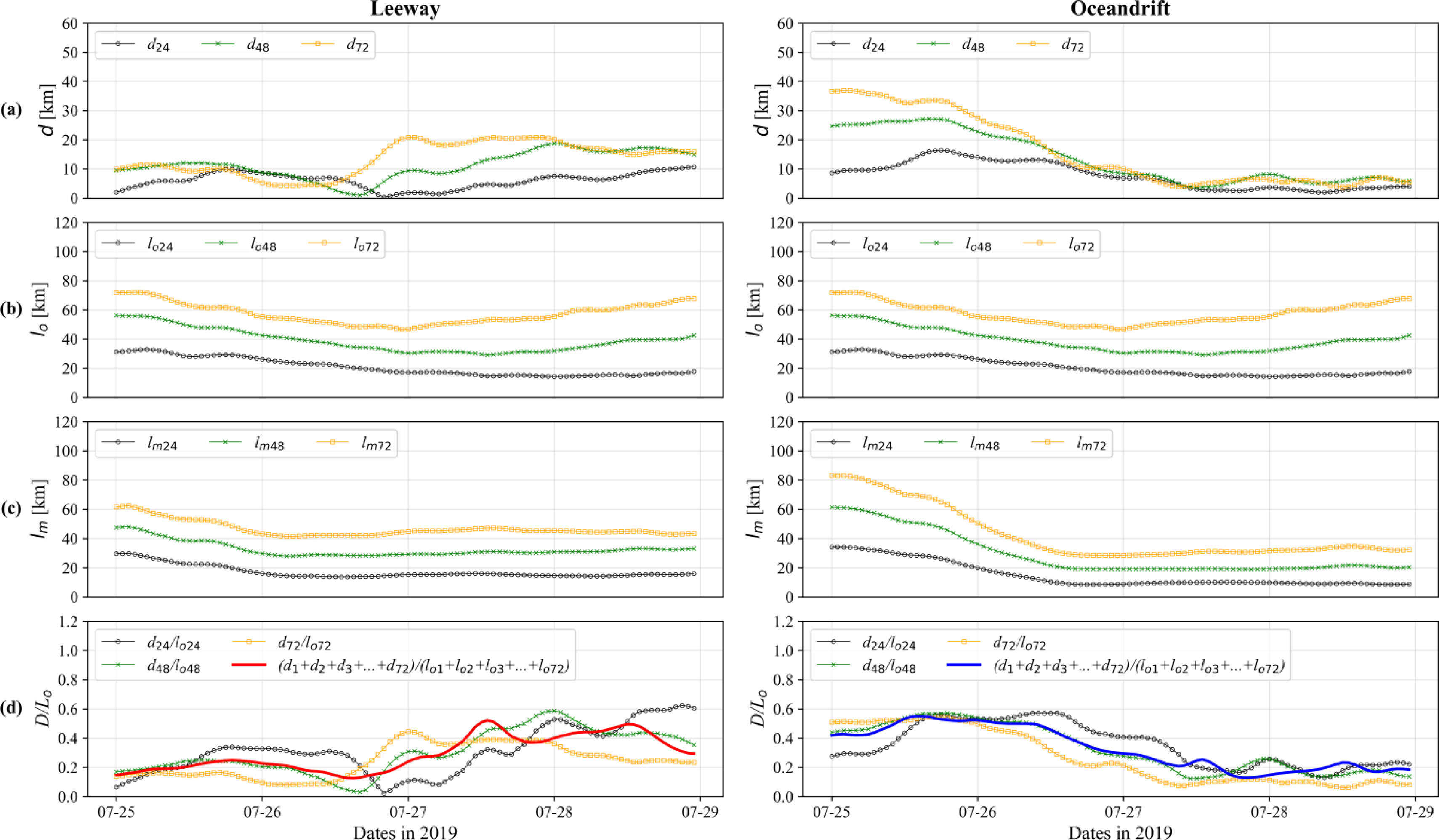
Results of the NCLS analysis using OpenDrift. The left panel displays the analysis results from the leeway module, while the right panel shows those from the oceandrift module. The x-axis signifies the start time of the simulation. The black solid lines represent the calculated position 24 h after the start of the simulation, the green solid lines indicate the position 48 h after the start of the simulation, and the yellow solid lines show the position 72 h after the start of the simulation: (a) Distance discrepancy between the model and observations at each simulated time point; (b) Cumulative sum of the drifter’s travel distance (observation); (c) Accumulated total travel distance for each respective module; (d) Result of s calculation based on Eq. (4).
The results of the NCLS analysis based on the start time of the OpenDrift simulation showed that the leeway module demonstrated a high value of 0.8091 on average from the initial simulation start time of 0:00 on July 25 to 23:00 on July 26. It then showed a low value of 0.6040 on average from 0:00 on July 27 to 23:00 on July 28. The oceandrift module showed a low value of 0.5392 from 0:00 on July 25 to 23:00 on July 26 and a high value of 0.8000 on average from 0:00 on July 27 to 23:00 on July 28. Fig. 12 shows the spatial distribution of NCLS skill scores by location depending on the start time of the simulation. It shows that the predictive performance of the leeway module decreases when it is closer to land, while the oceandrift module’s predictive performance increases when it is closer to land. These results are attributed to changes in the regional characteristics of external forces acting on the drifting bodies (such as ocean currents and wind) as the drifter moves north and approaches the land, as well as the limitations of numerical model resolution, which pose challenges in accurately representing the intricate coastline of the southern coast of South Korea.

Spatial distribution of NCLS skill scores based on the simulation execution locations (72 h after results): (a) leeway and (b) oceandrift
4.3 Analysis of Usability in Maritime SAR
A polygonal area was generated by connecting the outermost points of the particles distributed every hour by OpenDrift, and the presence of drifters in this area was calculated for each simulation to compute the LPC. Fig. 13 shows the process of calculating LPC for the leeway module and the oceandrift module when the simulation starts at 0:00 on July 25, 2019. In Fig. 13(a), the drifter is included in the leeway module’s predicted area while it is moving in the ENE direction, and it moves out of the predicted area as it moves north. It then reenters the area as it rotates near its final location. In Fig. 13(b), the drifter is included in the oceandrift prediction area in the initial few hours, but it deviates significantly from the prediction area afterward.
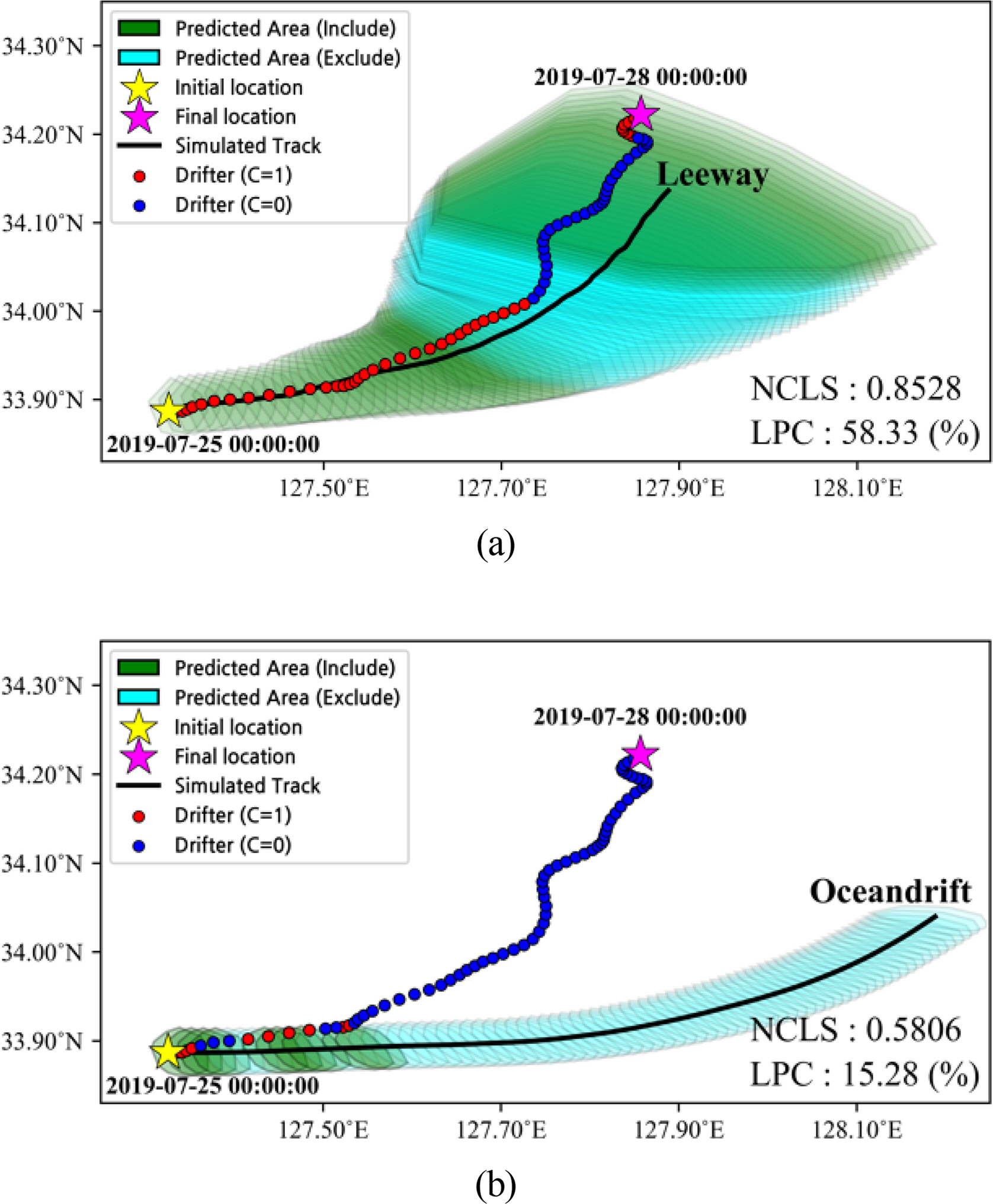
Results of LPC calculations based on the simulation elapsed time: (a) leeway and (b) oceandrift
The average LPC over the elapsed time was 100% for up to 2 h into all simulations and then decreased as more time elapsed. Notably, the LPC of the oceandrift module decreased sharply as more simulation time elapsed, ultimately reaching 0%. However, the leeway module’s LPC decreased as more simulation time elapsed and then maintained a certain level without a further decrease (Fig. 14). The average value for the entire elapsed simulation time was 53.51% for the leeway module and 16.50% for the Oceandrift module, indicating that the leeway module exhibited approximately 324% higher predictive performance than the oceandrift module.

Results of LPC calculations based on the simulation elapsed time (average across all simulations)
According to Tipton et al. (2022), considering a typical scenario where a person in the water can survive for 14 h, the average performance during a 14-hour simulation period was found to be 79.54% for the leeway module and 48.96% for the oceandrift module. The leeway module exhibited approximately 162% higher prediction performance compared to the oceandrift module. Furthermore, the results at the 14-hour mark showed that the LPC was 69.79% for the leeway module and 15.63% for the oceandrift module. In this case, the leeway module demonstrated approximately 447% higher prediction performance compared to the oceandrift module (Table 5). The LPC score represents the probability of drifters being located within the predicted area of OpenDrift and consistently showed higher performance for the leeway module compared to the oceandrift module. Based on these findings, it is suggested that considering the leeway module is important when determining areas with a higher likelihood of maritime objects being present.
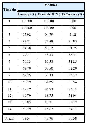
Results of LPC based on the simulated elapsed time (1–14 h)
5. Conclusions
Unlike terrestrial distress, maritime distress necessitates swift and accurate location estimation as drifting objects gradually move away from the incident site. Taking into account the distinctive characteristics of maritime emergencies, which is characterized by significant uncertainties and potential human and property losses, this study employed OpenDrift to conduct drift trajectory prediction experiments. Specifically, the leeway module of OpenDrift, which accounts for the crucial leeway effect in maritime SAR operations, was utilized. A comparative analysis of the leeway module and the oceandrift module, which solely relies on ocean current information without considering the leeway effect, was performed. To assess the performance of OpenDrift, four evaluation methods, namely NCLS, RMSE, MAE, and Euclid, were employed to gauge the congruence between the actual drift trajectories and the simulation results. Furthermore, an LPC analysis was conducted to evaluate the practicality of OpenDrift in maritime SAR scenarios. The key findings derived from this study can be summarized as follows:
(1) The evaluation of drift trajectory prediction performance in OpenDrift simulations revealed that both the leeway module and the oceandrift module exhibited decreasing prediction performance with elapsed simulation time. After 72 h of simulation, the results of the leeway module showed higher scores in all evaluation metrics on average. However, when considering the error range, no significant difference was observed. Therefore, it can be concluded that there are limitations to assessing the prediction performance of simulations including leeway using this approach.
(2) The NCLS analysis results based on the simulated locations in OpenDrift showed variations in prediction performance depending on the initial locations. The leeway module yielded a high average value of 0.8091 when the simulation started from July 25th at 0:00 to July 26th at 23:00. However, when the simulation started from July 27th at 0:00 to July 28th at 23:00, the average value dropped to 0.6040. However, the oceandrift module exhibited a low average value of 0.5392 when the simulation started from July 25th at 0:00 to July 26th at 23:00 and a relatively high average value of 0.8000 when the simulation started from July 27th at 0:00 to July 28th at 23:00. This can be attributed to the changing regional characteristics of external forces acting on the drifting objects, such as ocean currents and wind, as the drifter moves northward and closer to the land. Additionally, it is considered that the limitations of the numerical model resolution used in OpenDrift simulations in accurately representing the complex coastline of the southern coast of South Korea contributed to these results.
(3) Finally, in the LPC analysis, which evaluated the usability of the OpenDrift simulation results for maritime SAR, the leeway module showed average prediction performance that was approximately 324% higher than that of the Oceandrift module. Furthermore, when considering the maximum survivable time for a person in the water in general situations, which is 14 h, the leeway module exhibited approximately 447% higher prediction performance compared to the oceandrift module. Therefore, this study suggests that considering the leeway effect in drift trajectory prediction experiments can lead to higher probabilities of drifters being present within a predicted area, thereby enhancing the applicability of such predictions in maritime SAR operations.
This study confirmed that considering the leeway effect can be helpful in predicting areas with a higher likelihood of containing the actual locations of maritime drifting objects during drift trajectory prediction. The results of this study were quantitatively presented. Therefore, these findings can be utilized in evaluating and improving drift trajectory prediction techniques employed by maritime SAR organizations such as the KCG and KHOA. Additionally, these results are expected to have applicability beyond maritime disasters and can be extended to the prediction of drift trajectories for other floating objects, including marine debris, satellite buoys, and sea ice.
In future research, it will be necessary to use numerical model data with higher resolution to accurately simulate the intricate coastline of South Korea. Additionally, conducting field experiments to more accurately simulate the leeway effect on the target drifters would further enhance the usability of research results. However, it should be noted that this study was limited to the Korea Strait. By conducting OpenDrift research considering the characteristics of various maritime areas in South Korea, which is surrounded by sea on three sides, and validating them based on real maritime distress cases, it is believed that it can greatly contribute to future maritime SAR operations.
Notes
Sungwon Shin serves as an editorial board member of the Journal of Ocean Engineering and Technology, but he had no role in the decision to publish this article. No potential conflict of interest relevant to this article is reported.
This research was partially supported by the Korea Institute of Marine Science & Technology Promotion (KIMST), which is funded by the Korea Coast Guard (20220463), and by the Korea Evaluation Institute of Industrial Technology (KEIT) grant, which is funded by the Korean government (KCG, MOIS, NFA) [RS-2022-001549812, Development of technology to respond to marine fires and chemical accidents using wearable devices].