


1. Introduction
Ocean wave predictions are made using numerical wave models that calculate the spectrum changes caused by the growth and dissipation of wave energy, mainly using spatial-temporal wind data as input. Numerical wave models can be divided into first-generation, second-generation, and third-generation models according to the number of source terms in their governing equations. Studies on predicting or simulating waves have mainly used third-generation numerical wave models, such as Simulating Waves Nearshore (SWAN), Wave Watch III, and Wave Model (WAM), which solve an action density balance equation to calculate the wave spectrum. Previous studies have developed more accurate simulations of parameters, such as significant wave height and peak period, and have improved modeling performance. Regarding studies on wave prediction in the waters around Korea, Kang et al. (2015) and Eum et al. (2016) employed the SWAN third-generation numerical wave model to simulate waves in the waters around the Korean peninsula using weather forecasting data provided by the European Centre for Medium Range Weather Forecasts (EMCWF) and Japanese Meteorological Agency (JMA) as input data.
Lee et al. (2010) used SWAN to simulate storm waves occurring on the east coast of Korea during winter, and Chun et al. (2014) developed a modified version of WAM for use in shallow waters and simulate storm waves occurring on the east coast. Do and Kim (2018) and Caires et al. (2018) simulated large-height swell-like waves on the east coast of Korea during winter using SWAN and the energy dissipation term coefficient calibration method for white-capping proposed by Rogers et al. (2003). Large-height swell-like waves occur when strong extratropical cyclones develop in strong winds on the East Sea during winter. As the resulting storm waves approach the coast, they develop into waves with a long period (approximately 9ŌĆō15 seconds) and large height (3 m or more) (Oh et al., 2010). The wind input data used for this include the spatial-temporal wind data from Weather Research and Forecasting (WRF) the ocean weather forecast systemŌĆÖs model (Park et al., 2015), Regional Data-Assimilation, and Prediction System (RDAPS) and Local Data-Assimilation and Prediction System (LDAPS) forecast models used for operational meteorological forecasting by Korean Meteorological Agency (KMA). Lee and Ahn (2018) simulated waves in the Yellow Sea and East China Sea using SWANŌĆÖs energy dissipation term coefficient calibration method for white-capping. Also, KMA is currently operating a wave forecast system (global, regional, and local coastal model), which was built based on Wave Watch III.
Recently, hazardous large-height swell-like waves have repeatedly struck the east coast of Korea in winter (OctoberŌĆōFebruary) and have caused many instances of human and property damage. Since 2005, the number of diseased and missing persons due to large-height swell-like waves has reached 70, and the scale of property damage has exceeded an annual average of 10 billion KRW (Lee et al., 2014; Oh et al., 2010). To improve the forecast accuracy for hazardous waves that occur on the east coast of Korea during winter, this study performed numerical simulation of waves using SWAN, a third-generation numerical wave model that is used worldwide, and the Source Term 6 (ST6) developed by Rogers et al. (2012) by calculating physical coefficients based on recent field observations. The results of this study were compared to results obtained using the existing empirical formula created by Komen et al. (1984). As the input wind data for the numerical wave model, this study used data from RDAPS, which is KMAŌĆÖs operational meteorological model, ECMWFŌĆÖs latest 5th generation re-analysis model (ERA5), and the JMA meso-scale model (JMA-MSM). RDAPS data can be downloaded in real-time through KMAŌĆÖs Open MET Data Portal (http://data.kma.go.kr), and the JMA-MSM data were procured from JMAŌĆÖs database. The ERA5 data were obtained using Python and the application programming interface provided by ECMWF. In this study, the operational meteorological modelŌĆÖs results and wind data generated as re-analysis data were used as input to the SWAN to simulate the waves that occurred on the East Sea from November 2016 to February 2017. The model results were compared with wave observation data from 6 locations on the open seas operated by KMA and the Korea Hydrographic and Oceanographic Agency (KHOA), and an optimization study was performed to improve the accuracy of the numerical model through error analysis.
2. Numerical Model
2.1 Simulating Waves Nearshore (SWAN)
This study performed numerical simulation of wave on the East Sea during the winter from November 2016 to February 2017 using SWAN (Booij et al., 1999), a numerical wave model developed at Delft University of Technology in the Netherlands. With its numerical models, SWAN is capable of considering the wave propagation from wind-induced wave growth, refraction, shoaling, reflection, and diffraction. Simultaneously, it can also consider deformation caused by nonlinear wave actions (triad/quadruplet waveŌĆōwave interactions) as well as the wave energy dissipation caused by white-capping, breaking, and bottom friction. SWANŌĆÖs governing equation is a wave action balance equation that expresses waves in the form of a directional wave spectrum and calculates energy spectrum changes in a 2D horizontal space as follows:
where ╬Ė is the direction, and Žā represents each frequency, expressed as 2ŽĆ/f. N is the wave action density spectrum, where the wave energy spectrum is divided by each frequency and is expressed as N =E (Žā,╬Ė)/Žā. cx,cy,c╬Ė,cŽā are the wave energy propagation speeds at each phase (x,y,╬Ė,Žā). on the right side is a source term that shows the generation and reduction of wave energy density caused by wind, nonlinear wave actions, white-capping, bottom friction, and breaking as follows:
Sin is the growth in wave energy caused by the wind. Snl3 and Snl4 are the terms for energy dissipation caused by triad/quadruplet wave-wave interactions, respectively. Sds,w, Sds,b, and Sds,br are the terms for energy dissipation caused by white-capping, bottom friction, and depth-induced wave breaking, respectively. White-capping is a breaking phenomenon caused by wave steepness on the open ocean, and it is difficult to describe with an equation due to its strong nonlinear behavior and turbulence phenomena; as such, it is determined by an empirical equation. In SWAN, the term for energy dissipation caused by white-capping (Sds,w ) is expressed by HasselmannŌĆÖs (1973) pulse-based model, where the wave number (k) becomes a variable, as shown in Eq. (3) (WAMDI Group, 1988):
where Žā╠ā and k╠ā are the mean of each frequency and mean wave number, respectively, and ╬ō is the coefficient resulting from the total wave steepness, as shown in Eq. (4):
where Cds is the energy dissipation coefficient, ╬┤ is the white-capping weight value with respect to the wave number, s╠ā is the total wave steepness, s╠āPM is the total wave steepness of the PiersonŌĆōMoskowitz spectrum, which is
3.02 ├Ś 10 - 3
2.2 Sea Surface Wind Data
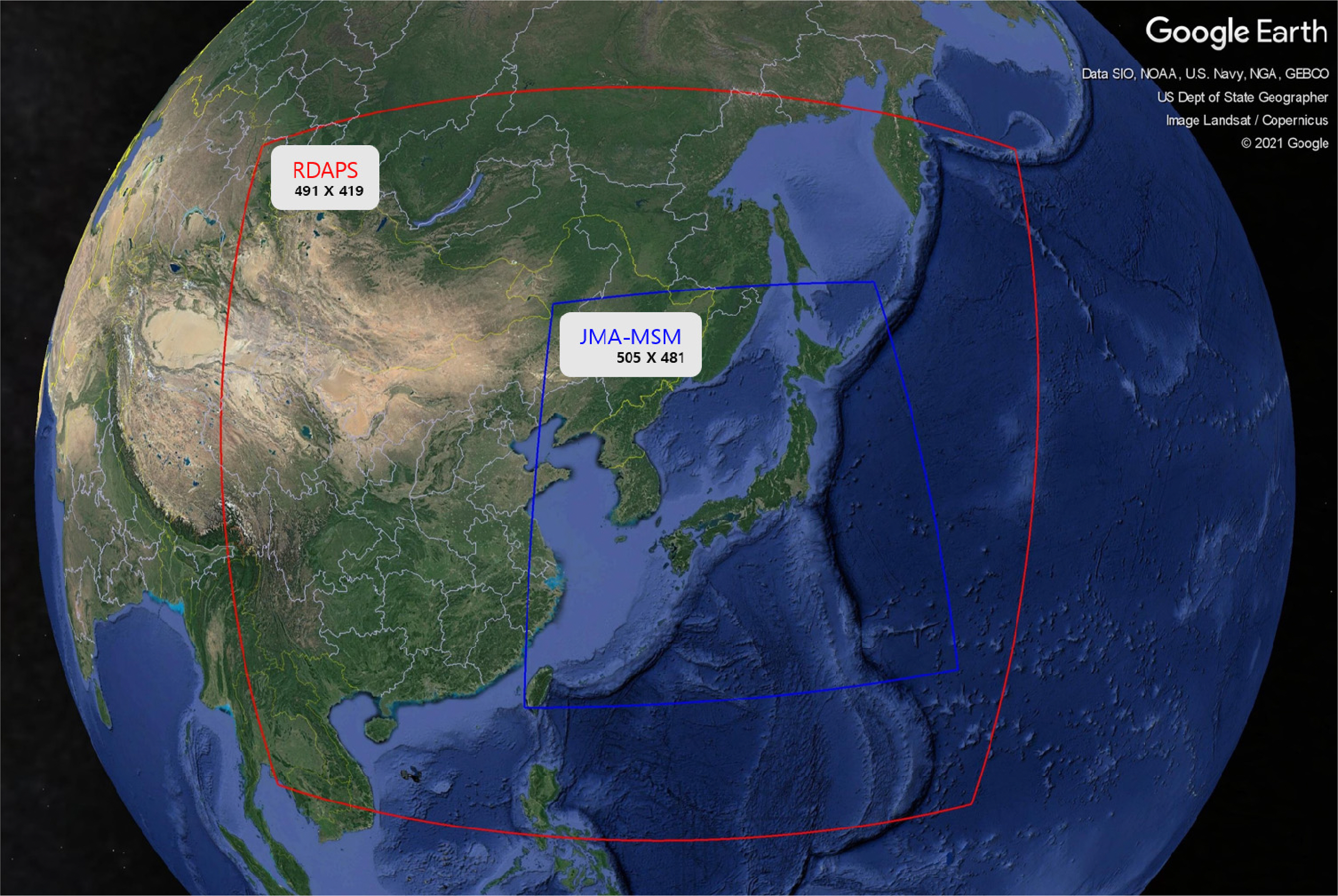
Numerical wave models use spatial-temporal sea surface wind data as input. Because data for the entire scope of the ocean are required, the results of numerical weather forecast models are used. As input wind data for its numerical simulation of waves on the East Sea, this study used wind data from RDAPS, which is operated by KMA, JMA-MSM, and ERA5. The ERA-Interim data provided by ECMWF have a temporal resolution of 6 h, which is considered limited for simulating waves that occur during rapidly changing severe weather (Do and Kim, 2018). The ERA5 single-level sea surface wind data, which have a temporal resolution of 1 h, were used for the input conditions of the numerical simulation of waves. RDAPS uses four-dimensional variational data assimilation (4D-Var) and is operated alongside LDAPS. Although LDAPS has a higher spatial-temporal resolution than RDAPS at 1.5 km and 3 h, it has limitations regarding numerical simulation of waves on the East Sea because its modeling area is limited to the area around the Korean peninsula, and it does not include the entire East Sea. Also, according to Do and Kim (2018), there is no great difference between the wave simulation results obtained by combining the results of LDAPS and RDAPS and the wave simulation results obtained using results of RDAPS alone; therefore, this study used RDAPS. The JMA-MSM (Saito et al., 2006) wind data are the product of a meso-scale weather forecast model operated by JMA and have a high spatial-temporal resolution. As such, these data have been used as input data in previous studies on numerical simulation of waves in the waters around Korea (Kim et al., 2020; Kwon et al., 2020; Yoon et al., 2020). Table 2 lists the spatial-temporal resolution, area, and data provision period for the 3 models used as input wind data in this study. To summarize the characteristics of each set of wind data, the RDAPS data have better spatial resolution than ERA5; however, at 3 h, its temporal resolution is lower than that of ERA5 and JMA-MSM. ERA5 has fairly poor spatial resolution, but it has a temporal resolution of 1 h, which allows for the analysis of rapidly changing weather conditions during severe weather, making it highly useful. JSM-MSM has a higher spatial resolution (5 km) than the other two models, and it has the advantage of providing the same 1 h temporal resolution as ERA5. Fig. 1 shows the operating range and grid numbers for the RDAPS and JMA-MSM input wind data used in this study. ERA5 is not shown as it is a global model.
2.3 Physical Coefficients, Grid, and Water Depth
The calculation area of the model constructed in this study was set as an equidistant grid with a 0.05┬░ ├Ś 0.05┬░ resolution containing the entire East Sea, including the Sea of Okhotsk, to model the development, propagation, and dissipation of storm waves caused by wind. The numerical modelŌĆÖs water depths are based on ETOPO1 (https://www.ngdc.noaa.gov/mgg/global/), which are satellite bathymetry data provided by the United StatesŌĆÖ National Oceanic and Atmosphere Administration (Fig. 2(a)). When the modelŌĆÖs grid was generated, the range of the weather data provided by JMA-MSM did not include the northern part of the Sea of Okhotsk, and the model grid for this area was modified as shown in Fig. 2(b). To closely model the periodic components of long-period waves, such as large-height swell-like waves, this study divided the wave energy spectrum frequency into 41 parts from 0.03 to 1.5 Hz and divided the wave direction into 48 parts in 7.5┬░ intervals to calculate the wave energy spectrum. Also, the additional physical parameters required to operate the SWAN model were set as listed in Table 3.
3. Numerical Wave Model Scenarios and Model Parameters
This study analyzed wave observation data with a focus on the winter season, in which large-height swell-like waves occur with great frequency. The numerical simulation period was set as November 2016 to February 2017, a period when a large number of large-height swell-like waves occurred.
For the numerical simulation of waves method, the ST6 proposed by Rogers et al. (2012) was applied to the East Sea numerical wave model. For the parameters in the model, combinations of the 4 parameters listed in Table 1 were used to simulate large-height swell-like waves, and these were compared with observation data for validation. Also, research was performed on optimizing the numerical wave model by comparing its results with the results of a simulation that uses an empirical equation by Komen et al. (1984), which is currently the default setting for SWAN. In this study, the model results were divided according to the parameter settings and the input wind data provided by each different organization (RDAPS, ERA5, and JMA-MSM). Table 4 gives an overview of the names, input wind data, model settings, and parameters of the simulation scenarios considered in this study.
As the wave observation data for validating and optimizing the numerical model, this study used data from the KHOAŌĆÖs ocean observation buoys (Northeast of Ulleungdo, E01; Northwest of Ulleungdo, E02) and KMAŌĆÖs open sea buoys (East Sea, DH; Ulleungdo, URD; Pohang, PH; Uljin, UJ), and Fig. 3 shows the locations and water depths of each observation buoy. In this study, the significant wave height and peak wave period data observed at each location were used to analyze the accuracy of the numerical wave model. To judge the model accuracy in detail, this study used wave observation data that had undergone primary data quality validation by Wave Information Network of Korea (Jeong et al., 2018).
4. Validation and Analysis of Numerical Model Results
In this study, the ST6 and parameter settings, which were developed to improve the numerical wave model proposed by Rogers et al. (2012), were used in simulation of winter waves occurring on the East Sea, and the forecast accuracy regarding significant wave height and peak wave period was evaluated. As mentioned previously, data provided from Korea, Japan, and Europe were used to verify the consistency of the modelŌĆÖs results according to the spatial-temporal input wind data. The results were compared with the results of simulations that use the empirical equation by Komen et al. (1984), which is the default setting of the SWAN model. In addition, the simulation results using the wind data provided by different organizations were compared to evaluate the simulation results regarding their input wind data. To quantitatively verify the simulation results, a statistical analysis of the difference between the model results and observation data was performed. The model evaluation items used for this analysis included the bias, root mean square error (RMSE), correlation coefficient (Žü), and index of agreement (IOA), as given by Eqs. (8)ŌĆō(11), respectively:
where n is the number of observation data, M is the modelŌĆÖs result value, O is the observed value, M╠ä and O╠ä are the respective mean values of M, O . In the statistical analysis, a comparison was made between the observed values and model results over a 1 h interval only in cases where the values in the observed significant wave height time series data during the interval were Ōēź1.0 m. This was done to systematically evaluate the actual prediction accuracy by removing the observation data error that occurs when wave height is low.
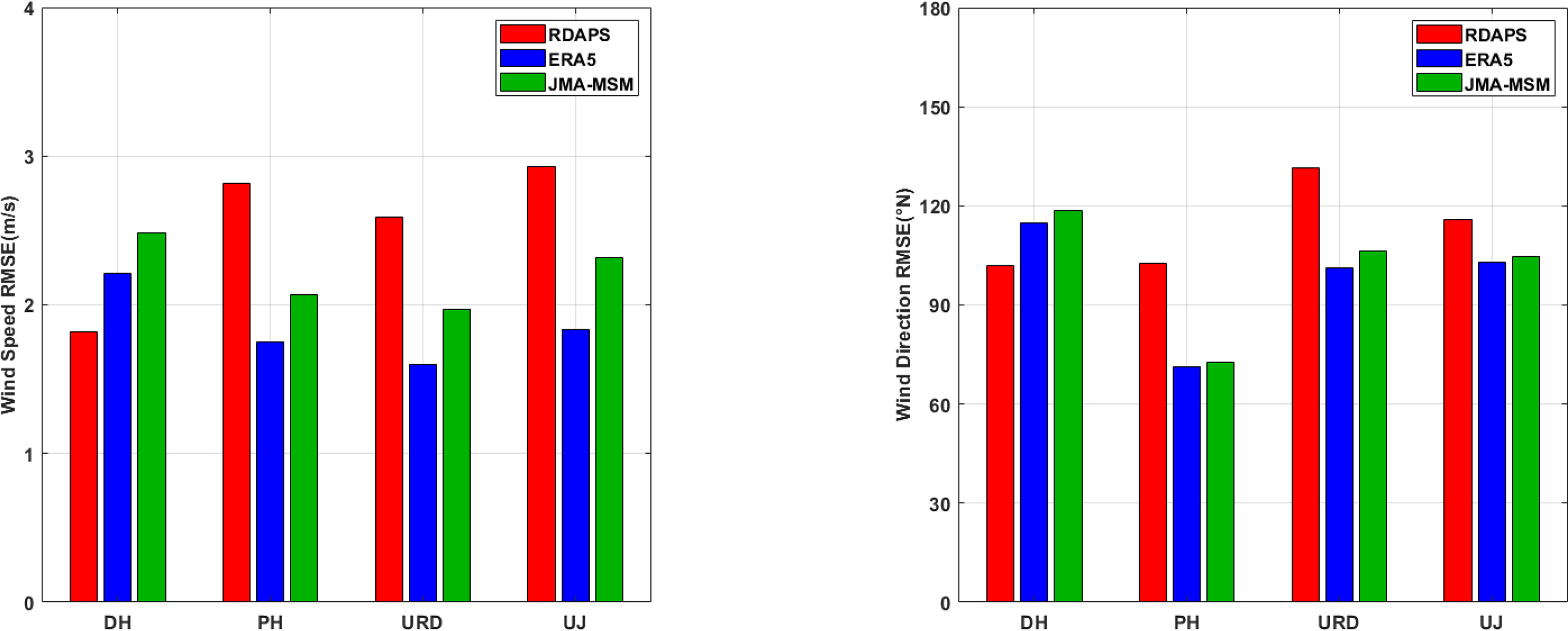
First, to evaluate the accuracy of the weather forecast data used as input to the numerical wave model, the wind speed and wind direction observed at the locations in Fig. 3 were compared to the input wind data, and the RMSE values for each weather model were plotted in a bar graph (Fig. 4). In the comparison process, the 2017 wind data from the KHOA-operated ocean observation buoys E01 and E02 were missing, and the data from the KMA-operated weather observation buoys DH, PH, URD, and UJ were used. When the data were analyzed, the ERA5 wind speed and wind direction had high overall accuracy, but the RDAPS forecast model had the lowest error at the DH. In the case of wind direction, there was no great difference in accuracy between the wind data produced by JMA-MSM and ERA5. In the case of wind speed, the accuracy of JMA-MSM was found to be excellent considering that it is a forecast model (Fig. 4 shows that JMA-MSMŌĆÖs wind speed had a higher RMSE of approximately 0.5 m/s than ERA5, which is re-analysis data.).
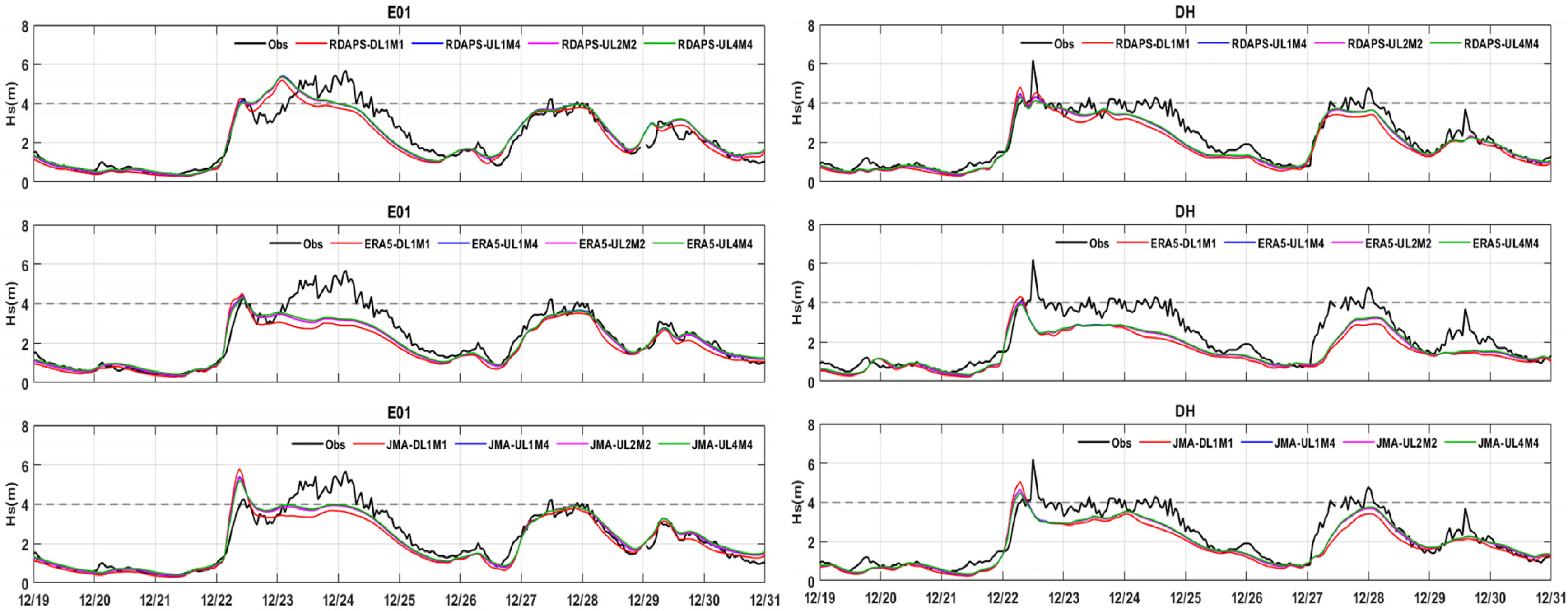
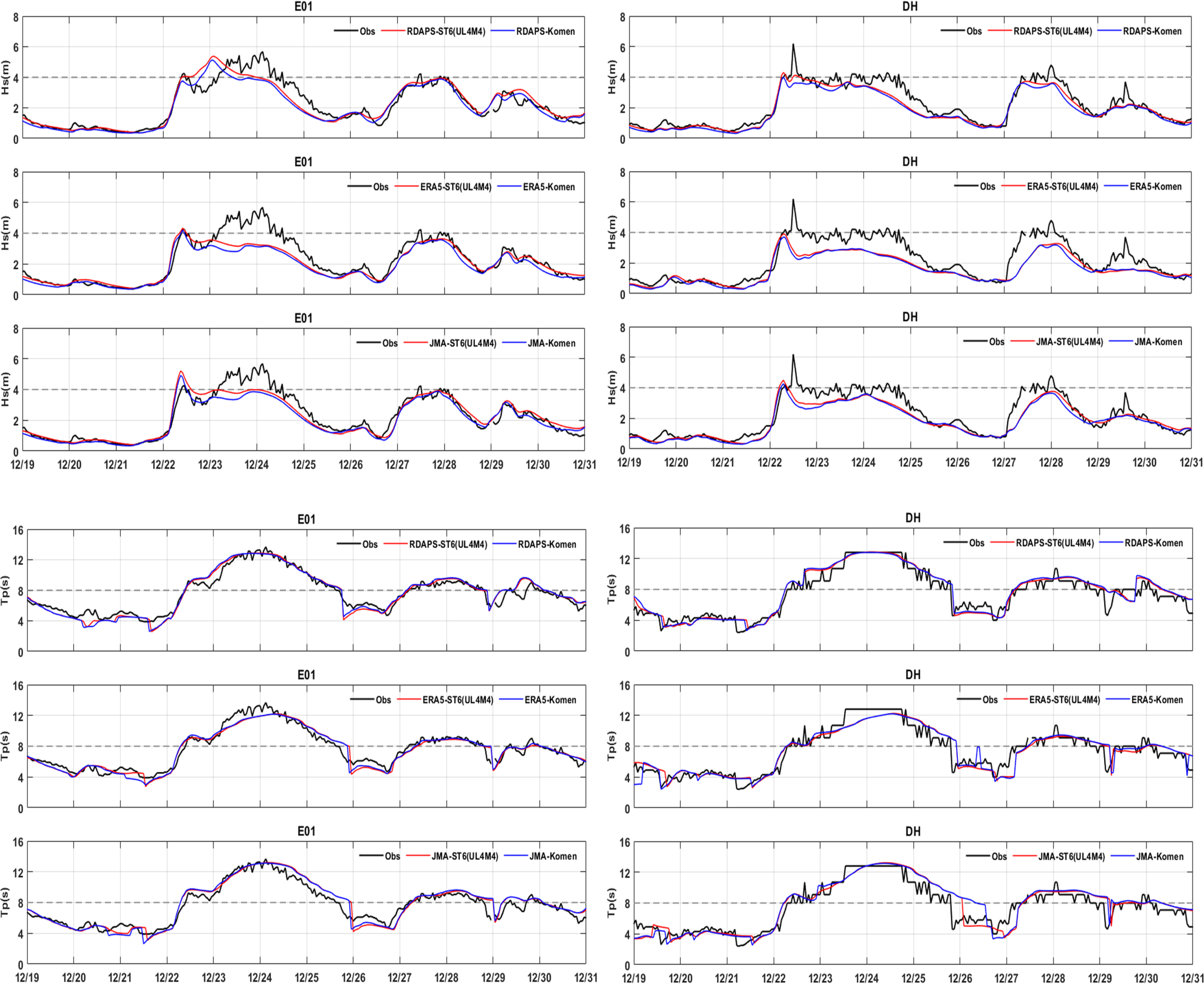
To find the input wind data and model composition that are most suitable for simulating large-height swell-like waves on the east coast of Korea in winter, significant wave height results for each simulation scenario were quantitatively analyzed, and the error statistics are listed in Table 5. It can be seen that the significant wave height simulation results from the ST6 configured with the UL4M4 parameter combination had the lowest error (RMSE of 0.02ŌĆō0.18 m) and the highest correlation coefficient and IOA, regardless of the input wind data. In contrast, when the DL1M1 parameter combination was used with the ST6, the simulation accuracy was the lowest. Fig. 5 shows a time series of the observation data and the significant wave height simulation results for each location predicted using the UL4M4 parameters, which had the highest accuracy of all parameter settings (RDAPS/ERA5/JMA-MSM-UL4M4). To evaluate the forecast accuracy for hazardous waves that occur during severe weather, the ST6ŌĆÖs significant wave height simulation results using 4 parameter settings (DL1M1, UL1M4, UL2M2, UL4M4) were divided up according to the input wind data for December 19ŌĆō31, 2016, which was a period when the significant wave height observed values were 4 m or greater and the numerical modelŌĆÖs error was high, and this is shown in Fig. 6. Here, there was no great difference in the error values between the model and observation data for each of the observation locations; therefore, the E01 and DH were selected as representatives from among the KHOA and KMA observation locations, and their data are shown as time series. It can be seen that there was no great difference between the simulation results that used the 3 parameter combinations UL1M4, UL2M2, and UL4M4, excluding DL1M1. However, as Table 5 shows, the results using the UL4M4 parameters, which produced the best statistics, had the largest significant wave height estimates, and these results were close to the observed values. In contrast, the results obtained using the DL1M1 parameters, which showed the worst model results in Table 4, estimated the waves to be lower than for other settings. Looking at the significant wave height results for December 23 and 24 at E01 and December 28 at DH in Fig. 6, the results obtained using the 3 parameter settings UL1M4, UL2M2, and UL4M4 all showed the significant wave heights to be approximately 0.1ŌĆō0.2 m higher than when using DL1M1, regardless of the input wind data. However, looking at the results for December 22, when the observed significant wave height rapidly increased, the wave height estimated by the DL1M1 settings was the largest, contrary to the previous results. It is believed that this is because the DL1M1 parameter combination does not use the ST6, which employs the new value for calculating the coefficient of energy dissipation due to white-capping, and therefore DL1M1 shows somewhat different characteristics in the predicted process of wave development.
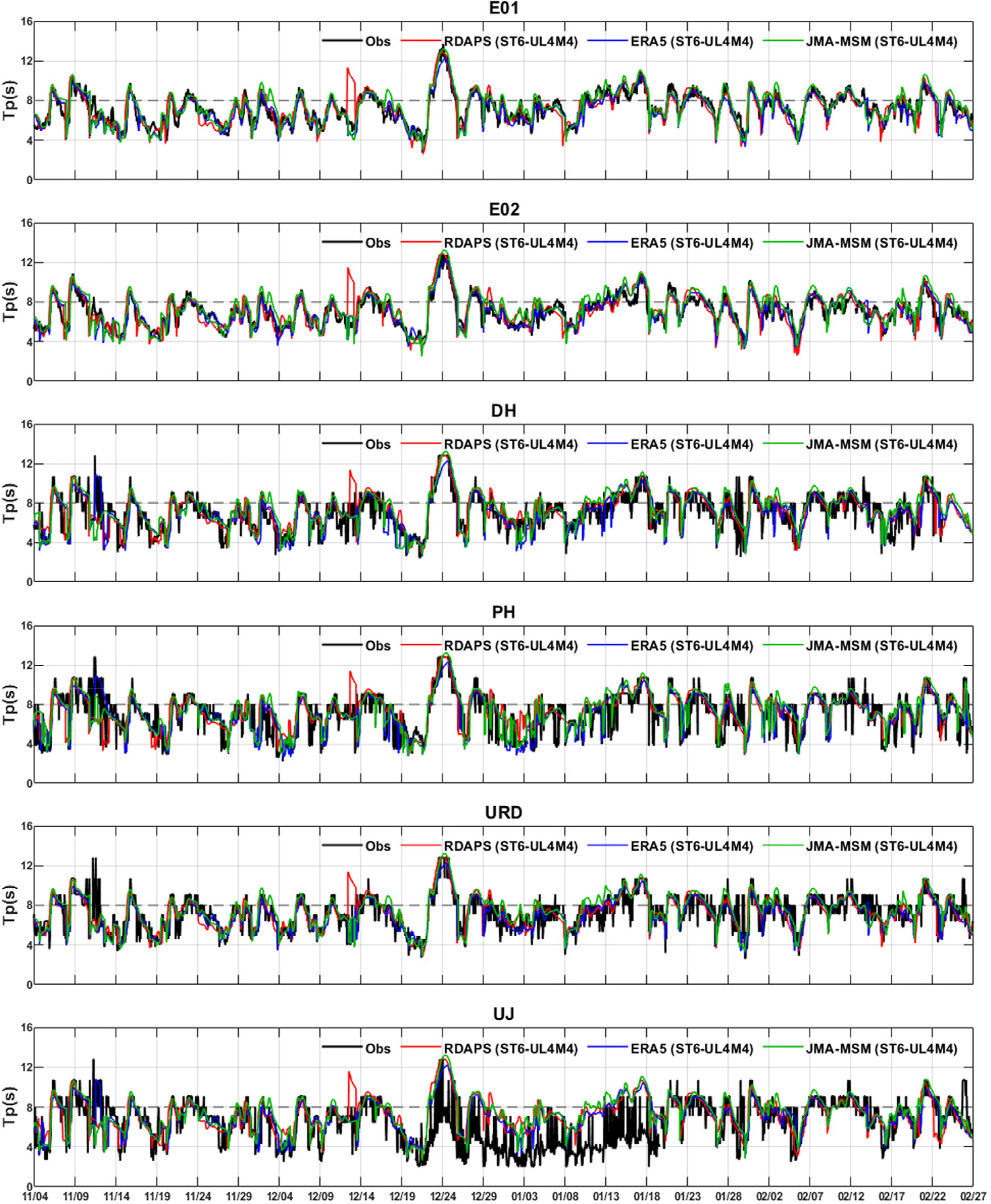
To analyze the simulation accuracy regarding wave period, Table 6 lists the statistics for error between the peak wave period results of this studyŌĆÖs numerical wave model and the observation data. From the simulation result statistics, it can be seen that there was poor consistency in the statistical comparative analysis results for the four ST6 models (DL1M1, UL1M4, UL2M2, UL4M4) for each combination of input data and observing locations used, and it is difficult to distinguish the model with the best results. All of the peak wave period model results for the KMA observing location UJ had very poor reproducibility, with a correlation coefficient of less than 0.51. Fig. 7 shows the peak wave period simulation results at each observing location for the ST6 models that showed the best reproducibility for significant wave height (RDAPS/ERA5/JMAMSM-UL4M4) along with the observation results in a time series. As can be seen in the figure, the model was not able to simulate the observed peak wave periods at UJ from December 20, 2016 to January 18, 2017. It is believed that an observation error occurred because the peak wave period values observed at UJ at that time were somewhat smaller than at other observing locations, and in the future, it will be necessary to examine the wave data quality management and data analysis methods to identify the cause of the error.
To examine the ST6ŌĆÖs wave prediction improvement effect, this study compared ST6ŌĆÖs simulation results to simulation results that use the empirical equation by Komen et al. (1984), which is the default setting for the SWAN model. Time series data for December 19 and 31, 2016 at E01 and DH are shown in Fig. 8. It can be seen that the two simulation results show no great difference in terms of peak wave period; however, in the case of significant wave height, ST6 predicted the wave height to be somewhat higher overall compared to the results obtained using the empirical equation by Komen et al. (1984). The difference between the two methodsŌĆÖ results is clear between December 22 and 24, when a large significant wave height occurred and temporal variability was high. Looking at the statistical analysis values listed in Table 4, it can be seen that RDAPS/ERA5/JMA-UL4M4 had an RSME that was lower by a maximum of 0.1 m and a lower deviation than RDAPS/ERA5/JMA-Komen, and the IOA and correlation coefficient were the same, or slightly higher for UL4M4. Thus, the simulation results using the empirical equation by Komen et al. (1984) were more accurate than the results of the ST6 using the DL1M1 setting; still, they were less accurate than when using the other settings, i.e., UL1M4, UL2M2, and UL4M4. This shows that, depending on the settings, the ST6 can predict significant wave height more accurately than the empirical equation by Komen et al. (1984). However, this study targeted only some periods when swell-like waves occurred. As such, it will be necessary to examine the numerical wave modelŌĆÖs suitability for waves that occur in various weather conditions (large-height swell-like waves, storm waves, etc.), and it is believed that the wave prediction accuracy can be improved further by providing optimal parameters based on such an examination.
This study used various numerical simulation scenarios to find that the ST6ŌĆÖs UL4M4 parameter setting had the highest reproducibility for large-height swell-like waves that occur on the East Sea. Ultimately, this study evaluated the accuracy of numerical wave models according to the input wind data provided different organizations. Fig. 9 shows bar graphs of the RMSEs and correlation coefficients of the significant wave height and peak wave period simulation results of the model with UL4M4 settings using the wind data provided by RDAPS, ERA5, and JMA-MSM. These graphs examine the accuracy of the numerical simulation of waves according to the input wind data. It can be seen that the simulation results for significant wave height using the ERA5 wind data as input had the highest correlation coefficient, except in the case of the location DH. This is because the ERA5 wind data were created through later re-analysis, unlike the other wind data, which shows that the accuracy of the input wind data plays an important role in the simulation of significant wave height. However, the ERA5 simulation results had a higher RMSE than the simulation results from JMA-MSM at all other locations except for E01 and E02, and they had a higher RMSE than the simulation results from RDAPS at the DH, PH, and UJ. It can be said that when the ERA5 wind data were used as the input wind data, the overall significant wave height reproducibility was excellent, but accuracy was poor when simulating large-height waves with great temporal variability. This can be seen in Fig. 6, which shows Fig. 5ŌĆÖs simulation results in detail around both February 22 and December 24 at E01 and DH. The wind data provided by the ERA5 model are based on a global model, and while their temporal resolution is excellent compared to the RDAPS and JMA-MSM data, their spatial resolution is poor. Therefore, it is believed that the spatial resolution of the input wind data plays an important role in simulating hazardous large-height waves that rapidly increase and change during severe weather. Looking at the simulation results for peak wave period, except at the UJ, which had a correlation coefficient of less than 0.5, it can be seen that the lowest RMSE and highest correlation coefficient were obtained when using the ERA5 wind data, which had a high overall accuracy. Also, the RMSE for the peak wave period simulation results appears to be similar to the wind speed and wind direction RMSEs in Fig. 4, and it is believed that the accuracy of the wind speed and wind direction prediction has a large effect on predicting the periodic components of waves.
5. Conclusions
This study used SWAN, a third-generation numerical wave model that is the most widely-used model in the field of coastal engineering, and ST6, which incorporates physical coefficients created based on observational research, to build and optimize a numerical wave model that can be applied to the East Sea during winter. To evaluate the reproducibility of the ST6, the numerical wave model was run using 4 different parameter combinations (DL1M1, UL1M4, UL2M2, and UL4M4) that were verified by Rogers et al. (2012) and spatial-temporal wind data (RDAPS, ERA5, and JMA-MSM) provided by various organizations as input, and the parameter settings with the best reproducibility were found. The results were compared to those obtained using the empirical equation by Komen et al. (1984), which is the default option in the SWAN model. In addition, a comparison was made between the simulation results obtained using the spatial temporal wind data provided by each organization, and the reproducibility of the simulation results was evaluated according to the input wind data.
Looking at the ST6 models with the 4 different parameter settings, it was found that the significant wave height reproducibility was best when using the UL4M4 parameters, and it was possible to obtain higher reproducibility by adjusting the parameters compared to using the empirical equation by Komen et al. (1984). In the case of peak wave period, there was poor consistency in the results according to each model, observing locations, and evaluation item, and it was difficult to evaluate reproducibility. When looking at the simulation results obtained by using each organizationŌĆÖs wind data, which had different characteristic, it was found that the best simulation results for significant wave height and peak wave period were obtained by using the ERA5 wind data. However, when predicting hazardous waves with great temporal variability, large wave heights were better simulated by RDAPS and JMA-MSM wind data, which are forecast models with worse wind speed accuracy but better spatial resolution than ERA5. This confirmed that the input wind dataŌĆÖs spatial resolution quality has a greater effect on wave prediction than wind speed accuracy when predicting large-height waves great temporal variability.
Ultimately, it was confirmed that ST6 can simulate the waves that occur in the East Sea to a certain extent by using various parameter settings instead of the empirical equation by Komen et al. (1984) used in existing numerical wave models. Also, it is believed that wind data with excellent spatial resolution quality are required to predict hazardous waves, which are characterized by large heights and occurrence during severe weather. Therefore, it will be possible to build a numerical wave model that can be applied to the entire East Sea by using a nesting method on the coastal areas. However, this study was not able to properly simulate significant wave heights that rapidly increased by more than 4 m and which occurred on December 19ŌĆō31, 2016, January 8ŌĆō18, 2017, or around February 21, 2017. There was an error of approximately 1 m in the simulation results for the location URD around January 20 and at locations DH, PH, and UJ around January 30. This means that third-generation numerical models, which calculate the wave energy spectrum using a wave action density equilibrium equation, are limited in predicting hazardous waves, such as storm waves and large-height swell-like waves that occur during typhoons and periods of severe weather. As such, it will be necessary to continue studying simulations for waves that occur in various environments, including severe weather conditions, and it will be necessary for data assimilation, which are used to increase prediction accuracy in the field of meteorology, to be applied to wave predictions to overcome the limitations of hazardous wave prediction.