A ship rudder is regarded as a continuum with infinite degrees of freedom. Unlike the equation of motion of an object with a finite number of degrees of freedom, the Lagrange equation based on the variational approach is required to derive the equation of motion of a continuum structure. The vibration of a continuum structure for an external force can be obtained using the Lagrange equation as follows: where T, Γ, U, W, and q_j refer to kinetic energy, energy dissipation term, potential energy, work, and the jth degree of freedom displacement function, respectively.

The ship rudder can be assumed as a one-dimensional continuum structure. In addition, as the bending and twisting modes predominantly influence the ship rudder, the deformation z of the structure can be assumed as a function of time t and space x, as follows: where S_fj and S_gj are the jth mode bending and twisting shape functions, respectively; and d_j and θ_j are the jth mode bending- and twisting-mode coefficients, respectively. When the deformation of the structure is defined in this way, T and U are expressed as follows: where μ, EI and s refer to structural linear density, flexural rigidity, and span length, respectively. When Eqs. (3) and (4) are applied to Eq. (1), the motion equation in the form of a matrix is obtained, as follows: where M, C, K and F refer to structural mass matrix, structural damping matrix, structural elastic matrix, and external force vector, respectively.

The fluid force and moment exerted on the vibrating wing cross-section should consider the static fluid force and moment variation according to the angle of attack and the amplitude reduction and phase shift due to unsteadiness. The amplitude reduction and phase shift due to unsteadiness depend on the dimensionless frequency k of the wing cross-section, which is expressed by the Theodorsen function C(k) as where H12(k) and H02(k) are the Hankel functions of the second kind.

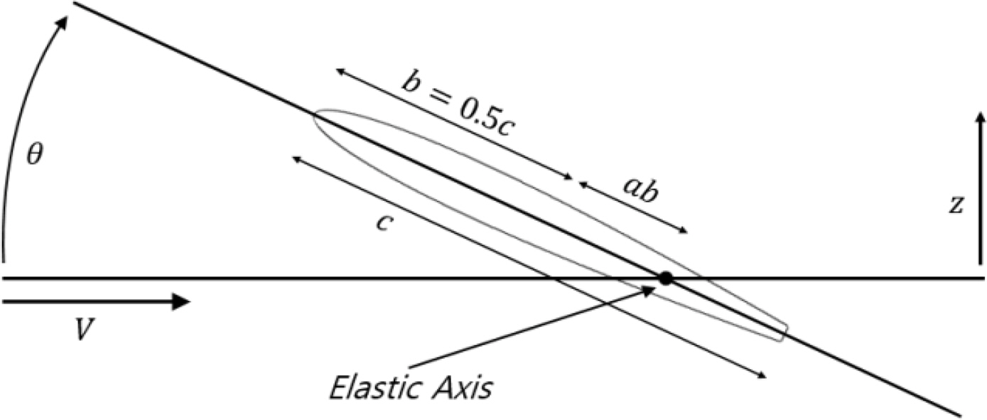
Theodorsen (1949) derived the fluid force and moment L_T, T_T exerted on the thin wing cross-section in flow velocities based on the potential method as follows: where ρ_f refers to the fluid density; a is the dimensionless distance from the midpoint of the chord to the elastic axis of the wing cross-section; b is half the chord length; and V, d and θ refer to the flow velocity, bending displacement, and twisting angle, respectively. The upward direction of d and L_T is positive, and the counterclockwise direction of θ and T_T is positive. A schematic diagram of a, b, c and V, and the directions of d and θ in the wing cross-section is shown in Fig. 1.

The potential method is based on the assumption of incompressible, inviscid and irrotational condition. In this study, we focused on predicting VIV when vortex shedding occurs in the wake of ship rudders. As vortex shedding occurs due to the viscosity and boundary layer of the fluid, it is theoretically impossible to predict the vortex strength and vortex shedding frequency based on the potential method. Therefore, CFD considering viscosity is essential for deriving the vortex-induced fluid force and moment. Chae (2015) developed a BT FSI analysis method for deriving the VIV of the hydrofoil using CFD. By considering only the first bending- and twisting-mode vibration of the hydrofoil, the bending displacement and twisting angle of the hydrofoil can be assumed, as in Eq. (9).

The equation of motion Eq. (10) is obtained applying Eq. (9) to the Lagrange equation Eq. (1) described in Section 2.1, as follows:

Here, where x_θ, r_θ, ω_b1, ω_t1, ξ and I_p refer to the distance from the elastic axis to the center of gravity, the radius of gyration, the first bending-mode natural frequency, the first twisting-mode natural frequency, the damping coefficient, and the polar moment of inertia, respectively; S_ff11 is the value obtained by integrating the square of the first bending-mode shape function S_f1 from 0 to s. In the same way, S_gg11, S_f″f″11 and S_fg11 are the values obtained by integrating the square of S_g1, S_f″1 and S_f1S_g1 from 0 to s, respectively. The loose-coupling method can perform the FSI analysis using Eq. (10) as the governing equation and applying the boundary conditions in Eq. (11) at the fluid-structure boundary interface. where ν^m, σ^s, σ^f and n refer to the mesh movement velocity, structural stress, fluid stress, and normal vector, respectively

F_CFD includes the inviscid force F_T = [S_ff11L_T, S_gg11T_T]^T based on the potential method. When the fluid density is much smaller than the structural density, the effect of the inviscid force of F_CFD is inconsiderable. Therefore, it is appropriate to perform the FSI analysis using the loose-coupling method based on Eq. (10). However, in an underwater environment, since the fluid density is quite high, the effect of the inviscid force by the added mass, added damping, and added stiffness is relatively considerable. Therefore, it is inappropriate to use Eq. (10) as the governing equation. Chae (2015) used Eq. (12), where the inviscid force term is excluded on both sides of Eq. (10), as the governing equation for the BT FSI analysis, to reflect the effect of the inviscid force in an underwater environment without subiterations in the partitioned method.

Here, where e and f are 2a + 1 and 2a − 1, respectively.

While the FSI described in Eq. (12) in the previous section has the advantage of favorably reflecting the effect of the inviscid force by the added mass, etc., without subiteration in an underwater environment, it also has a disadvantage in that it cannot realize resonance and lock-in phenomena caused by high bending- and twisting-mode vibration by taking into account only the first bending- and twisting-mode vibration. Therefore, in this study, we extend the governing equation for the FSI analysis to take into account high bending- and twisting-mode vibration. First, we extend the equation for the bending displacement and twisting angle, yielding

If the governing equation for FSI analysis that considers high bending-and twisting-mode vibrations is obtained by applying Eq. (13) to Eq. (1) and Eqs. (7) – (8), the equation can be written in the form of a matrix equation of size 2n × 2n for the nth mode. The derived matrix equation has regularity; thus, it can be generalized to a matrix pattern of size 2 × 2. The governing equation for the FSI analysis is expressed for a relatively simple second mode as follows:

Here, i,j = 1,2

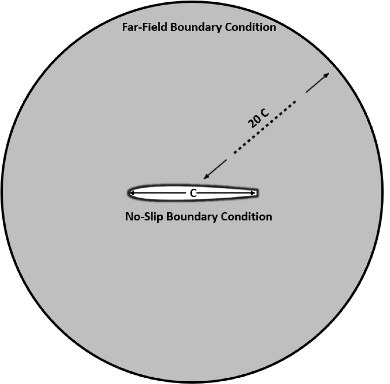
In the process of FSI analysis, we performed the CFD analysis of the hydrofoil by first identifying the reliability of the CFD analysis. In this analysis, we used OpenFOAM, an open-source CFD program. The CFD solver is based on the Reynolds-averaged Navier-Stokes (RANS) governing equation. The k− ω shear stress transport (k − ω SST) model combining the k − ω model and the k − ∊ model was used as the turbulence model (Kim et al., 2017). The detailed analysis settings are listed in Table 1. For comparison with the experimental results, the same cross-section shape as that of the test object of Ausoni (2009) and Zobeiri (2012) was used as the hydrofoil shape for analysis. The wing cross-section shape to be analyzed is shown in Fig. 2. It is the same as NACA0009; however, it is cut so that the end thickness is 3.22% of the chord length. The chord length of the hydrofoil for analysis is 0.1 m. For comparison with the experimental results (Ausoni, 2009; Zobeiri, 2012), we performed the CFD analysis for a total of 17 flow velocities ranging from 10 m/s to 26 m/s at an interval of 1 m/s. Considering the underwater environment, we set the medium density to 1000 kg/m³ and the kinematic viscosity to 1e⁻⁶ m²/s. The analysis domain is a circle with a radius of 20 times the chord length, where the elastic axis of the analysis object is set to be at the origin. The analysis domain and boundary conditions are shown in Fig. 3, and the analysis mesh is shown in Fig. 4. The number of meshes is approximately 100,000, and the dimensionless number y+ value related to the thickness of the mesh closest to the wall is approximately 1. By assuming a far-field condition, we applied freestream velocity and freestream pressure boundary conditions to the outer boundary of the analysis domain and applied a no-slip boundary condition to the wing surface. We used 5e⁻⁷ s as the time step, so that the maximum value of the Courant-Friedrichs-Lewy (CFL) number related to analysis stability did not exceed 1.

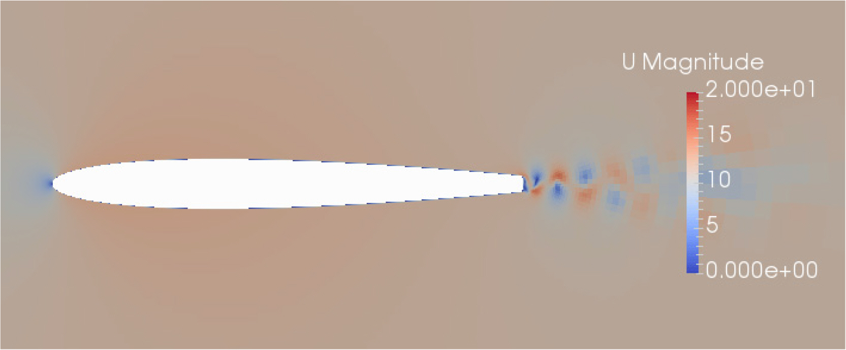
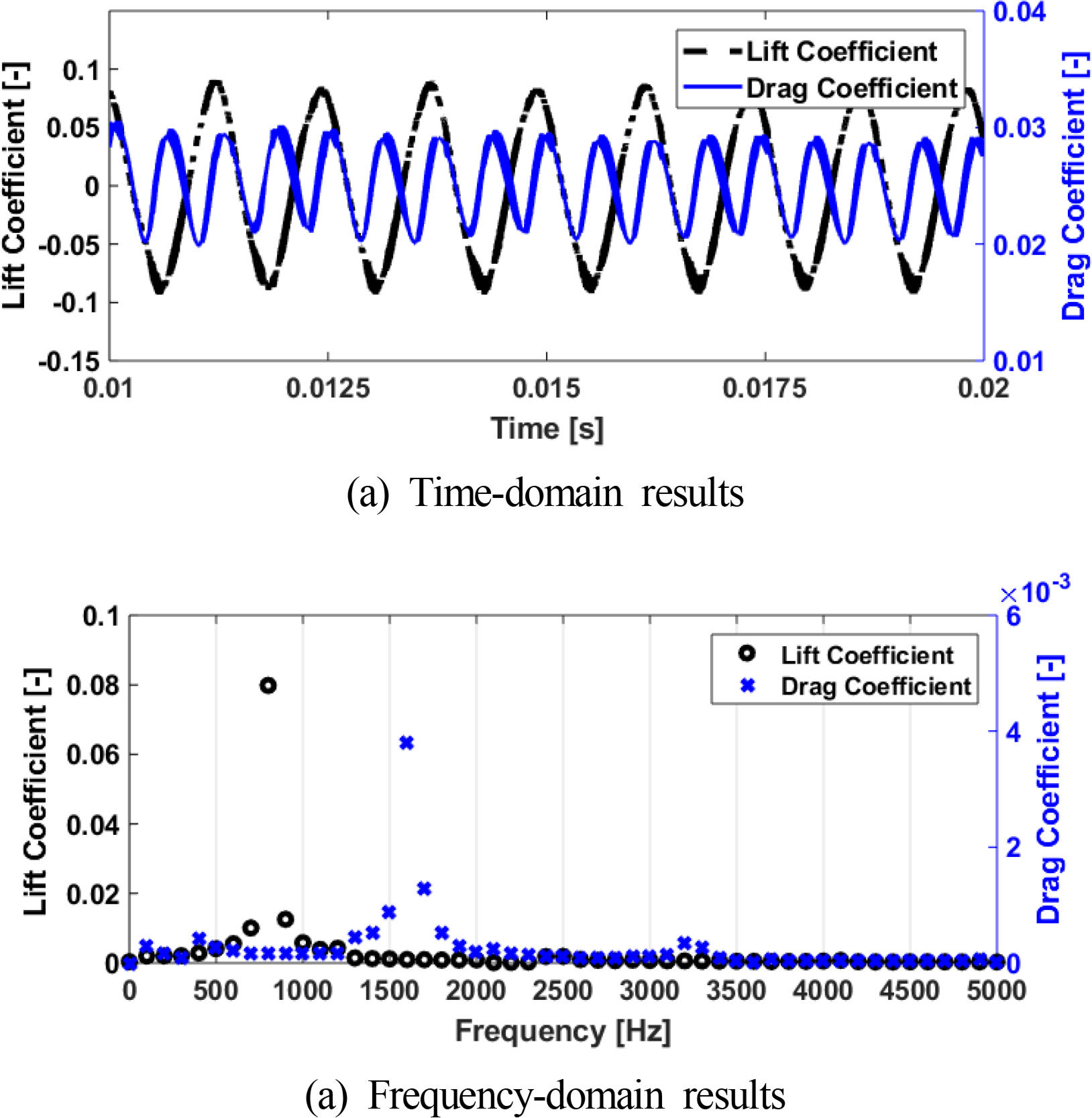
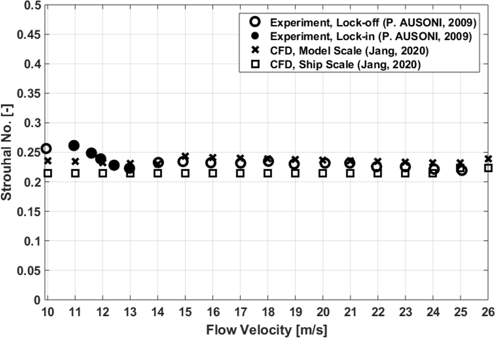
The CFD analysis result of the flow field around the hydrofoil is shown in Fig. 5, which confirms vortex shedding in the wake. The analysis results of drag and lift coefficients are shown in Fig. 6. Vibration characteristics of one dominant peak component are observed. In particular, the peak frequency of the drag coefficient is twice the peak frequency of the lift coefficient, which is attributed to the characteristics of vortex shedding that occurs alternately on both sides (Blevins, 2001). A comparison of the mean values of the drag and lift coefficients obtained using the experiment and the CFD analysis is shown in Table 2. For the drag coefficient, the analysis results differ from the experimental results by approximately 4% (Zobeiri, 2012); this is attributed to the difference in the 3D effect between the experimental and analysis results (Mittal and Balachandar, 1995). In addition, since this analysis model has a symmetrical shape with an angle of attack of 0°, the lift coefficient was approximately 0 in the experimental and analysis results. The Strouhal number of the hydrofoil for the flow velocity between the experimental and analysis results is shown in Fig. 7. The Strouhal number is a dimensionless number for the vortex shedding frequency f, and is defined as fD/V. Assuming that there is no resonance and lock-in, when D is set as the thickness between separation points, the Strouhal number is approximately 0.2 for a wide range of the Reynolds number regardless of the cross-section shape (Sarpkaya, 1979). The experimental results (Ausoni, 2009) show that the Strouhal number changes at the flow velocities of 10–14 m/s. This is because the vortex shedding frequency at these flow velocities is close to the structure’s natural frequency, thus causing resonance and lock-in phenomena. At the flow velocity after 14 m/s, the Strouhal number test result shows that it has a constant value of 0.23, and the Strouhal number derived by the CFD analysis (model scale, x) under the same Reynolds number has a constant value of approximately 0.24 in the entire flow velocity range, which is similar to the experimental results. We verified the reliability of this CFD analysis procedure by confirming that the lift coefficient, drag coefficient, and Strouhal number derived by the CFD analysis matches the experimental results.

To identify the characteristics of the fluid force frequency of the ship rudder, we performed the CFD analysis for each flow velocity on the model scale shape, enlarged 100 times, and represented the Strouhal number in Fig. 7 (ship scale, square). Despite a 100 times difference in the Reynolds number, the Strouhal number was approximately 0.22 in the entire flow velocity range, which is similar to the experimental and model scale analysis results and also matches Sarpkaya’s results (1979).

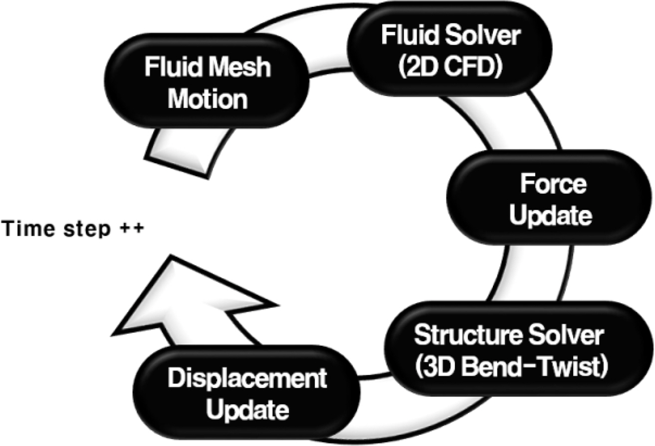
The high-mode BT FSI analysis procedure is shown in Fig. 8. For the CFD analysis, we used OpenFOAM, as in Section 3.1. The pimpleDyMFoam solver suitable for the analysis with mesh movement was used. The detailed analysis settings are listed in Table 3. The equation of motion Eq. (14) was used as the governing equation for the bending-twisting structural analysis.

To simulate the ship rudder, we set the analysis target to the model scale shape, enlarged 100 times, and created the CFD analysis using the same procedure as in Section 3.1. We applied freestream velocity and freestream pressure boundary conditions to the outer boundary of the analysis mesh domain and applied moving wall velocity boundary conditions to the wing surface, which satisfied Eq. (11). We used 2e⁻⁵ s as the time step, so that the maximum value of the CFL number related to analysis stability did not exceed 1.

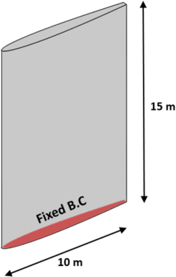
The structural parameter values required for the FSI analysis are shown in Table 4; ρ_s, EI, ξ, μ, and the center of gravity were derived for the shape, as seen in Fig. 9, and the material properties were derived for the steel structural model. Fixed boundary conditions were applied at the end of the model for the simulation of the ship rudder. The bending-mode natural frequency f_B, and the twisting-mode natural frequency f_T were derived using the 3D finite element method (FEM) to analyze the vibration for the structural model. When the twisting mode occurs, the position where the deformation was minimal was set as the elastic axis, and r_θ was derived based on this. The values related to the twisting-mode shape function were derived using the Euler-Bernoulli cantilever analytic solution (Abu-Hilal, 2003), and the first and second bending- and twisting-mode shape functions are shown in Fig. 10. It is expected that resonance and lock-in phenomena will occur in the first twisting mode and the second bending mode within the flow velocity range of this analysis; thus, we performed the BT FSI analysis considering the second mode as well.

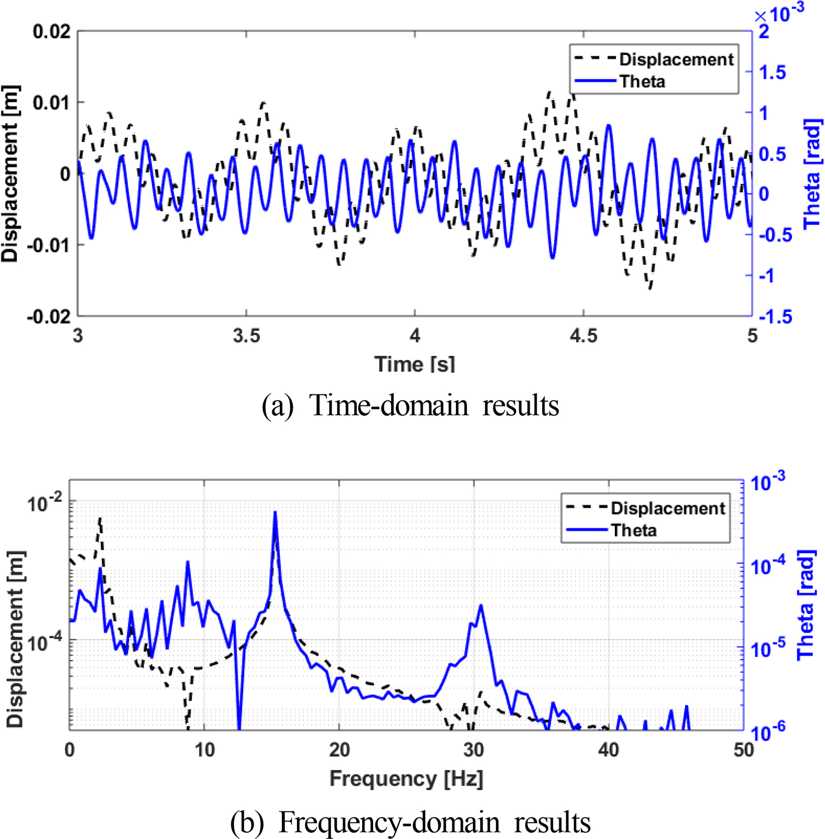
The vibration displacement and angle derived by the BT FSI analysis at a Reynolds number of 2.3e⁸ are shown in Fig. 11, and periodic vibration is observed in the figure. In particular, peak responses are observed in both the vortex shedding frequency component and the underwater natural frequency component. The VIV frequency for each flow velocity derived by high-mode BT FSI analysis of the hydrofoil is shown in Table 5. Overall, the VIV frequency tends to increase with an increase in the flow velocity. This is because the Strouhal number has a constant value in a wide range of the Reynolds number. We confirmed lock-in phenomena in which the VIV frequency was maintained at a constant value at flow velocities of 13–14 m/s and 23–24 m/s. We obtained the underwater natural frequency for the analysis target using the analytic solution of a cantilever (Ausoni, 2009), and compared this with the lock-in frequencies, as displayed in Table 6. The frequencies favorably matched the first twisting-mode underwater natural frequency and the second bending-mode underwater natural frequency, respectively, which confirm that 13–14 m/s was the first twisting-mode resonance and lock-in region; 23–24 m/s is the second bending-mode resonance and lock-in region. The underwater natural frequency is inversely proportional to the scale and the Strouhal number has a constant value in a wide range of the Reynolds number. Therefore, if the shape is the same, the lock-in velocity at which vortex shedding occurs at the underwater natural frequency, even when the scale is different, is the same as in Eq. 15 (Ausoni, 2009).

Here, V_lock, St and f_w are the lock-in velocity, Strouhal number, and underwater natural frequency, respectively. Using this, the 1/100 scale model experimental results (Zobeiri, 2012) were compared with the lock-in velocity. The lock-in velocity (11–13 m/s) obtained as a result of the experiment and the lock-in velocity (11–13 m/s) obtained as a result of the high-mode BT FSI analysis were similar, which verifies the reliability of this analysis in terms of the frequency.

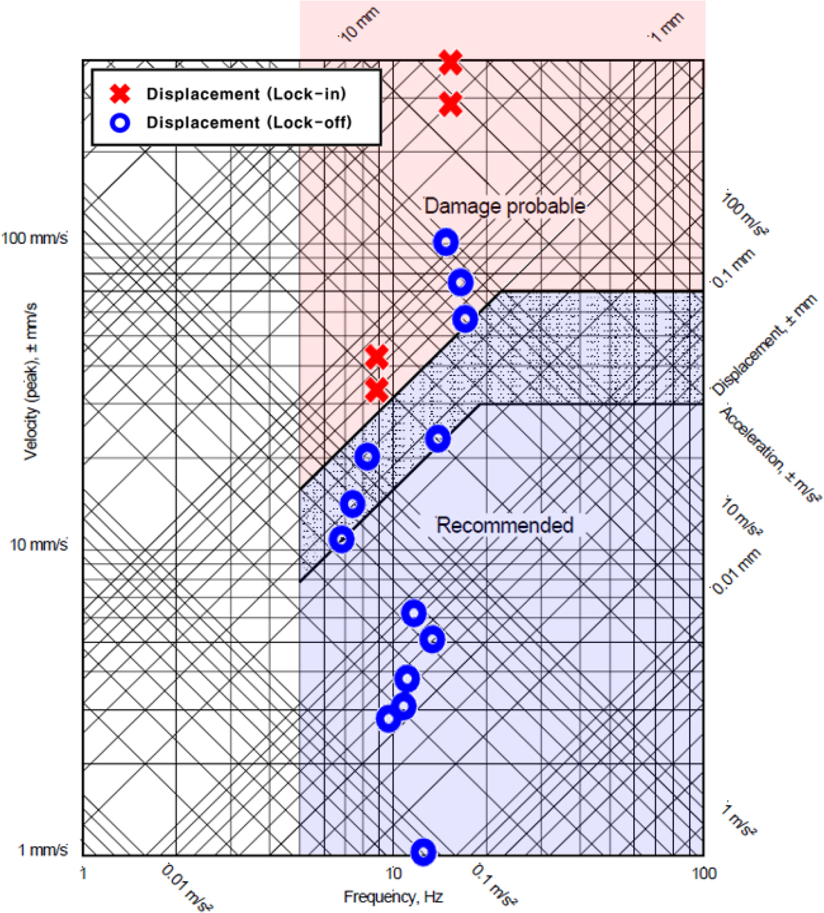
To examine the structural stability of ship rudders with the VIV responses derived through the analysis performed in this study, we referred to the local vibration guidance suggested by Lloyd’s Register (Lloyd’s Register, 2006). As seen in Fig. 12, the results of the VIV displacement derived using the high-mode BT FSI analysis are displayed in the ship’s local vibration guidance graph. The VIV responses displacement and frequency are shown in Table 5 and Table 7, respectively. An x in red indicates the displacement when lock-in occurs, and a circle in blue indicates the displacement in other situations. In the frequency range of interest (5–100 Hz), the red shaded area indicates the area where the risk due to vibration is expected to be high, and the other areas are shown as the blue shaded areas. The VIV responses in the lock-off condition was expected to cause a high risk at some flow velocities close to the second bending mode. The VIV responses in the first twisting mode and the second bending mode lock-in condition was expected to cause a high risk in terms of local vibration.