Behavior Characteristics of Density Currents Due to Salinity Differences in a 2-D Water Tank

Article information

J. Ocean Eng. Technol. 2018;32(4):261-271

Publication date (electronic) : 2018 August 30

doi : https://doi.org/10.26748/KSOE.2018.6.32.4.261

Woo-Dong Lee ^*

, Norimi Mizutani ^**

, Dong-Soo Hur^,^*

^*Department of Ocean Civil Engineering, Institute of Marine Industry, Gyeongsang National University, Tongyeong, Korea

^**Department of Civil Engineering, Nagoya University, Nagoya, Japan

Corresponding author Dong-Soo Hur: +82-55-772-9122, dshur@gnu.ac.kr

Received 2018 July 17; Revised 2018 August 8; Accepted 2018 August 13.

Abstract

In this study, a hydraulic model test, to which Particle Image Velocimetry (PIV) system applied, was used to determine the hydrodynamic characteristics of the advection-diffusion of saltwater according to bottom conditions (impermeable/permeability, diameter, and inclination) and the difference of the initial salt. Considering quantitative and qualitative results from the experiment, the characteristics of the density current were discussed. As an experimental result, the advection-diffusion mechanism of salinity was examined by the shape of saltwater wedge and the flow structure of density currents with various bottom conditions. The vertical salt concentration obtained from the experiment was used as quantitative data to calculate the diffusion coefficient that was used in the numerical model of the advection-diffusion of saltwater.

Keywords: Density current; Advection-diffusion; Salinity difference; Particle image velocimetry; Hydraulic model test

1. Introduction

Estuary is an area where the saltwater and freshwater meet together. Hence density current occurs due to the density difference of water mass. The combination of the currents due to horizontal pressure gradient under non-uniform density distribution and all the thermohaline circulations caused by temperature and salinity is called density current. For its characteristics, inrush depth is determined by the difference of fluid density and the reduced gravity (g‘) governs advection rate.

To analyze the characteristics of density current, many researches have been conducted by several methods: Theoretical (e.g. Shanack, 1960; Benjamin, 1968), experimental (e.g. Simpson, 1969; Huppert and Simpson, 1980; Marmoush et al., 1984), and observational (e.g. Wakimoto, 1982; Mueller and Carbone, 1987) studies were conducted to analyze the density current. Furthermore, Thomas et al. (1998) and Thomas et al.(2004) studied the density current propagating on porous layer through a hydraulic model experiment. Gray et al.(2006) studied propagation characteristic of density current on the slope, and Farhanieh et al.(2001) studied it numerically.

For 3-D researches, Lal and Rajaratham(1977) used a large water basin to study the characteristic of spatial distribution for temperature and velocity of the seas by warm water release. Natale and Vicinanza(2001) studied the effect of wave on the temperature distribution of neighboring seas, by warm water release. For the numerical researches, Paik et al.(2009) developed a 3-D model to simulate advection-diffusion of density current, and Firoozabadi et al.(2009) and Georgoulas et al.(2010) dealt with 3-D advectiondiffusion characteristics of density current through simulations. In addition, White and Helfrich(2008) numerically studied propagation characteristic of density current with wave excitation.

Meanwhile, according to the development of computer performance and numerical technique, many numerical models have been employed for the simulations in estuary. With these numerical models, characteristics of flow field of density current has been analyzed (e.g. Patterson et al., 2005; Cantero et al., 2006; Hormozi et al., 2008) and they are often applied to the sites out of experimental conditions (e.g. De Cesare et al., 2006; Sato et al., 2006).

In the numerical analysis of density current, it is important to calculate the material concentration, which affects fluid density, and advection-diffusion equation is applied to most numerical simulations in order to estimate the concentration. In the advection-diffusion equation, the advection terms, which are under absolute control of flow velocity, are dependent on a hydrodynamic model, but the diffusion terms are inevitably influenced by the diffusion coefficient in large amount. Therefore, it is important to estimate diffusion coefficient in the calculation of density current.

In the conventional numerical calculation without turbulence model, Richardson Number (R_i) that describes the stability in the fluid motion was used for the calculation (e.g. Blumberg, 1977; Pacanowski and Philanders, 1981). Currently, various turbulence models have been developed, and the eddy viscosity coefficient calculated from the turbulence model is generally used for the horizontal diffusion coefficient, and vertical diffusion coefficient is recalculated with application of Schmidt Number (Sc) or Prandtl Number (P_r), which is described as the ratio between the eddy viscosity and diffusion, according to the type of turbulence model, grid system, etc (e.g. Farhanieh et al., 2001; Lesser et al., 2004). In addition, Sato et al.(2006), who used the 3-D numerical model, selectively applied eddy viscosity coefficient calculated with large eddy simulation (LES) and diffusion coefficient that is calculated by substituting R_i and S_c.

This study covers the hydraulic model test for the advectiondiffusion of seawater according to initial salinity and bottom conditions (permeable/impermeableness, particle diameter and inclination). Through quantitative and qualitative analyses of the results, the characteristics of density current will be discussed. Furthermore, it will provide basic data for evaluating the diffusion coefficient applied to the numerical simulations for density current.

2. Experimental Setup and Procedure

2.1 Description of Hydraulic Model

Fig. 1 is a conceptual diagram of hydraulic model experiments with particle image velocimetry (PIV) system, and the water basin was fabricated with transparent acrylic panels for the basic experiment regarding to the density current. The water basin is 165 cm long, 20 cm wide, 40 cm high, and 25 cm depth, and it is divided into two compartments; one compartment is for the saltwater and the other one is for the freshwater. In Fig. 2, the water basins are filled with the saltwater and freshwater in the initial condition.

Fig. 1.

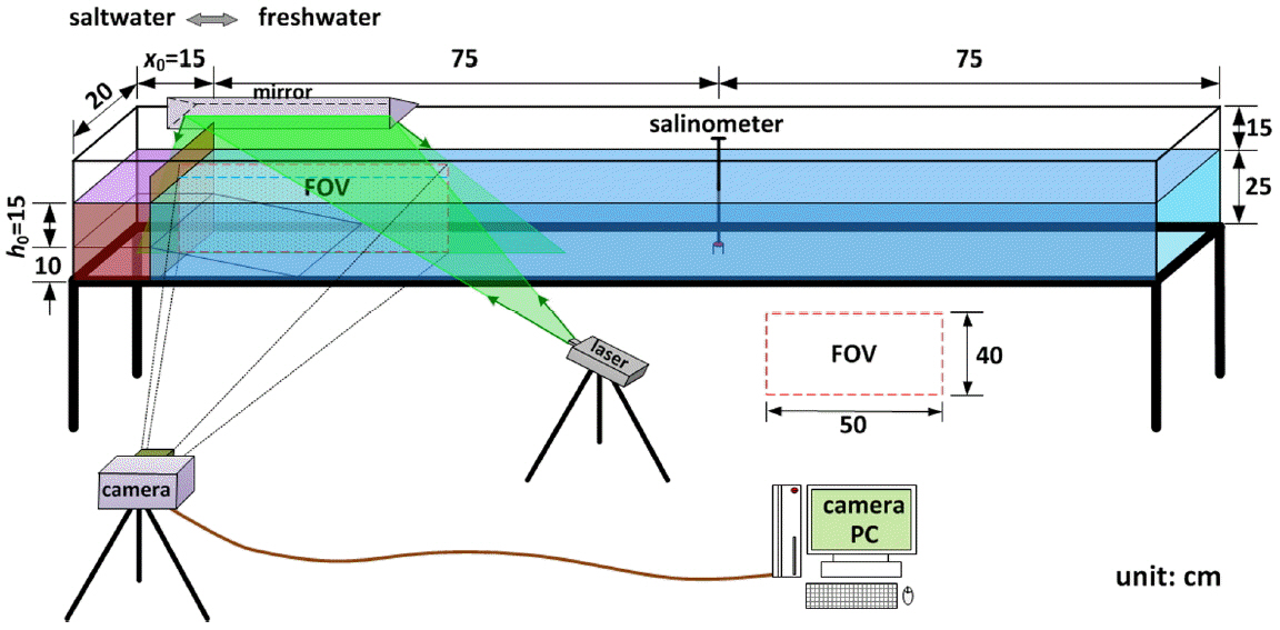
Schematic diagram of PIV system used in this study

Fig. 2.

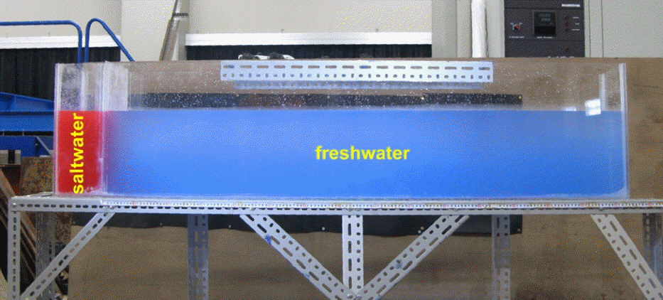
Setup of water basins for laboratory experiments

In density current experiments according to the bottom conditions, the water depth is 15 cm for the impermeable condition, and for the permeable condition (Fig. 3), the bottom of compartment is raised by 10 cm and the freshwater compartment is filled with sand or pebble with 10 cm thickness. Then, the water depth becomes 25 cm.

Fig. 3.

Composition of bed material in permeable bottom

For the experiment regarding to the bottom inclination, bed slope is considered from the compartment, as shown in Fig. 4. For the impermeable bottom condition, the bed slope is made of acrylic panels, and it is made of sand or pebble for the permeable bottom condition.

Fig. 4.

Setting of bed slope in water basin

The basic experiment about the density current for this study consists of watercolor experiment and PIV experiment, and the same experimental condition is repeated two times.

2.2 Experimental Conditions and Measurement

2.2.1 Experiment using Flow Visualization

In the flow visualization experiment, the saltwater is colored as shown in Fig. 3, and 39 cases of experimental runs are conducted. For this experiment, both bottom conditions of permeable and impermeable are considered, where average particle diameters (d_p) are 0.2 mm and 2.5 mm, and the inclinations (B_s) are 1:0 (cliff), 1:2, 1:3, 1:5 and 1:∞ (horizontal plane). The initial salinity is 10 psu, 20 psu, and 30 psu. In addition, the initial conditions are listed in Table 1 for the experiments related to the temperature, salinity and density of water. Here, the water density is calculated by empirical formula which was proposed by Gill(1982). S₀, T₀, and ρ₀ mean the salt, temperature and density of saltwater, and T_f and ρ_f mean the temperature and density of freshwater, respectively. g` is a reduced gravity and calculated as Δg/ρf (Δρ is the density difference between the saltwater and freshwater; and g is the gravitational acceleration).

Table 1.

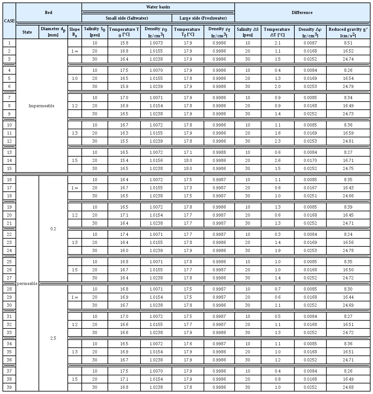
State of water and bed conditions used for watercolor experiments

In this experiment, the saltwater behavior according to advectiondiffusion of density current is captured with 1920pixel×108pixel camera in 0.04 sec interval. The salinity is measured on equilibrium of pressure (when the water is static with the flow velocity of 0 cm/s) after removing the partition, and it is measured at 75 cm away from the partition starting 0.5 cm from the bottom with 1 cm vertical interval.

2.2.2 Experiment using PIV System

The conditions for PIV experiment are the same as the watercolor one but the temperature condition, which has effect on the water density, is different. The temperature and density of water are shown in Table 2.

Table 2.

State of water and bed conditions used for PIV experiments

The PIV system for this study consists of a high-speed camera, computer to control the camera, laser to be lit on particles, mirror to control a laser sheet, and the particles equally mixed in the water. Here, the laser is a green laser sheet 1,000 m/G with wavelength of 3.52 × 10^-5 cm and the particles are high porous type synthetic adsorbents with specific gravity of 1.01 g/cm and effective size of 2.5 mm.

In this experiment, the movements of particles in 50cm×40cm area are recorded for 16.37 sec (1,637 frames at 100 frames/s) with a high-speed camera having the shutter speed of 1/2,000 sec and 1280pixel×1024pixel resolution. Then, a commercial software (DIPPFLOW^®) for 2-D fluid analysis is used for the particle video and the velocity component (u and w) is calculated in x-z direction for certain unit area of 32 pixel × 32 pixel (1.25 cm × 1.25 cm) with the resolution of 0.39 mm/pixel.

3. Experimental Results

3.1 Advection-Diffusion Characteristics of Saltwater

3.1.1 Characteristics due to Initial Salinity

Fig. 5 shows the advection-diffusion behavior of saltwater at 5 sec interval, according to the density (salinity) difference, and Fig. 5(a) is for the case that the initial salinity is 10 psu and Fig. 5(b) is for 30 psu. The red indicates saltwater, and black indicates freshwater. Where, h₀ is the initial depth and x₀ is the length of a compartment.

Fig. 5.

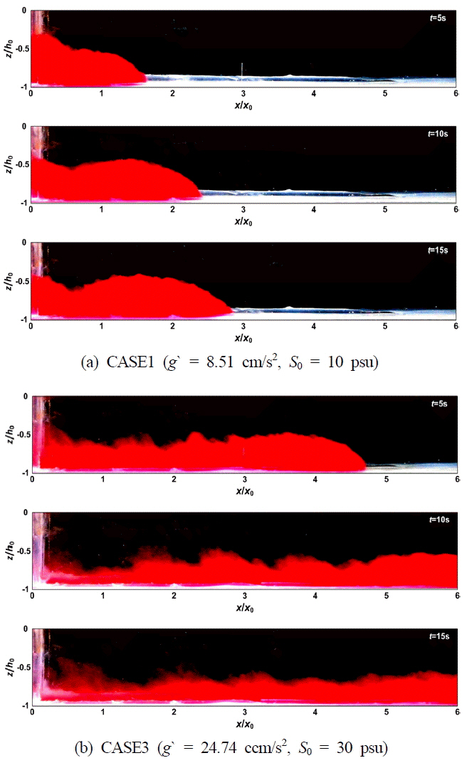
Advection-diffusion behavior of saltwater according to reduced gravity

In Fig. 5, when the initial salinity is high in the compartment, the density difference between saltwater and freshwater increases, resulting in higher g’, which affects the spreading rate. Thus, when g’ increases, the acceleration influencing the saltwater increases so that the advection speed of saltwater increases until the pressure gradient is balanced. In other words, bigger the density difference between the two fluids is, higher the reduced gravity resulting in faster movement of saltwater is. Comparing Figs. 5(a)-5(b), Karmann vortex occurs because of Kelvin-Helmholts instability when the reduced gravity (density difference) becomes higher. According to this, more saltwater spread is expected, and it will be discussed through the comparison and analysis of flow/vorticity fields and vertical salt concentration, which are obtained from PIV system.

3.1.2 Characteristics due to Components of Bottom

Fig. 6 shows the behavior of advection-diffusion of saltwater at 5 sec interval, according to the bottom conditions; Fig. 6(a) corresponds to the impermeable bottom; Fig. 6(b) to the permeable bottom with the mean diameter of 0.2 mm and porosity of 0.43; and Fig. 6(c) to the permeable bottom with the mean diameter of 2.5 mm and porosity of 0.41. In these cases, the initial salinity of compartment is S₀ 20 psu; the reduced gravity is g’ 16.52 cm/s²; the red indicates saltwater; and the black indicates freshwater.

Fig. 6.

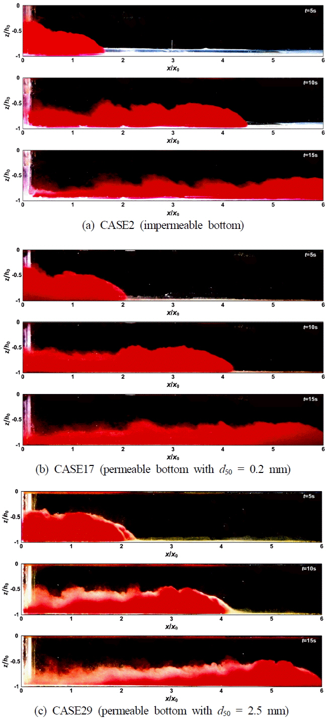
Advection-diffusion behavior of saltwater according to bottom conditions

The spreading rate of saltwater proceeding on the impermeable bottom in Fig. 6(a) is larger than those on the permeable bottoms of Figs. 6(b) and 6(c). It is not only due to bottom roughness but also the simultaneous effects from the shear force in/out side of permeable ground, due to some of water mass seeping into the permeable medium for the freshwater with the permeable bottom. So the spreading rate of saltwater decreases. With these, the spreading rate of saltwater decreases and the diffusion in the vertical direction is encouraged.

3.1.3 Characteristics due to Bottom Slope

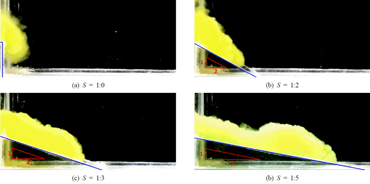
Fig. 7 shows the behavior of advection-diffusion of saltwater on the impermeable slopping bottom, at 2.5 sec interval; (a) is for the bottom slope of 1:2 and (b) is for the bottom slope of 1:3. Here, the yellow indicates saltwater and the black indicates freshwater.

Fig. 7.

Time series of contour shapes by advection-diffusion of saltwater over impermeable

In case of advection-diffusion of saltwater (see Figs. 5 ~ 6), the water mass is extended as the saltwater head moves. However, when it spreads along the slope as seen in Fig. 7, the size of head becomes large and shows oval shape as the head moves. In addition, during the saltwater is spreading along the sloping bottom, Kelvin-Helmholtz instability becomes weaker making relatively smooth boundary interface and Karmann vortex decreases. On the other hand, the backward distribution of saltwater mass (which went through the slopping bottom) becomes wider and it is considered that it occurs because of the congestion due to the speed difference with the tail when the flow velocity (which was accelerated while proceeding along the slopping bottom) becomes slower after it reaches to a flat bottom.

Fig. 8 shows the behavior of advection-diffusion of saltwater along the slopping permeable bottom of 1:3, with 2.5 sec interval; (a) is when the diameter of permeable medium is 0.2 mm and (b) is when the diameter of permeable medium is 2.5 mm. Here, the mint color indicates the saltwater and the black indicates the freshwater.

Fig. 8.

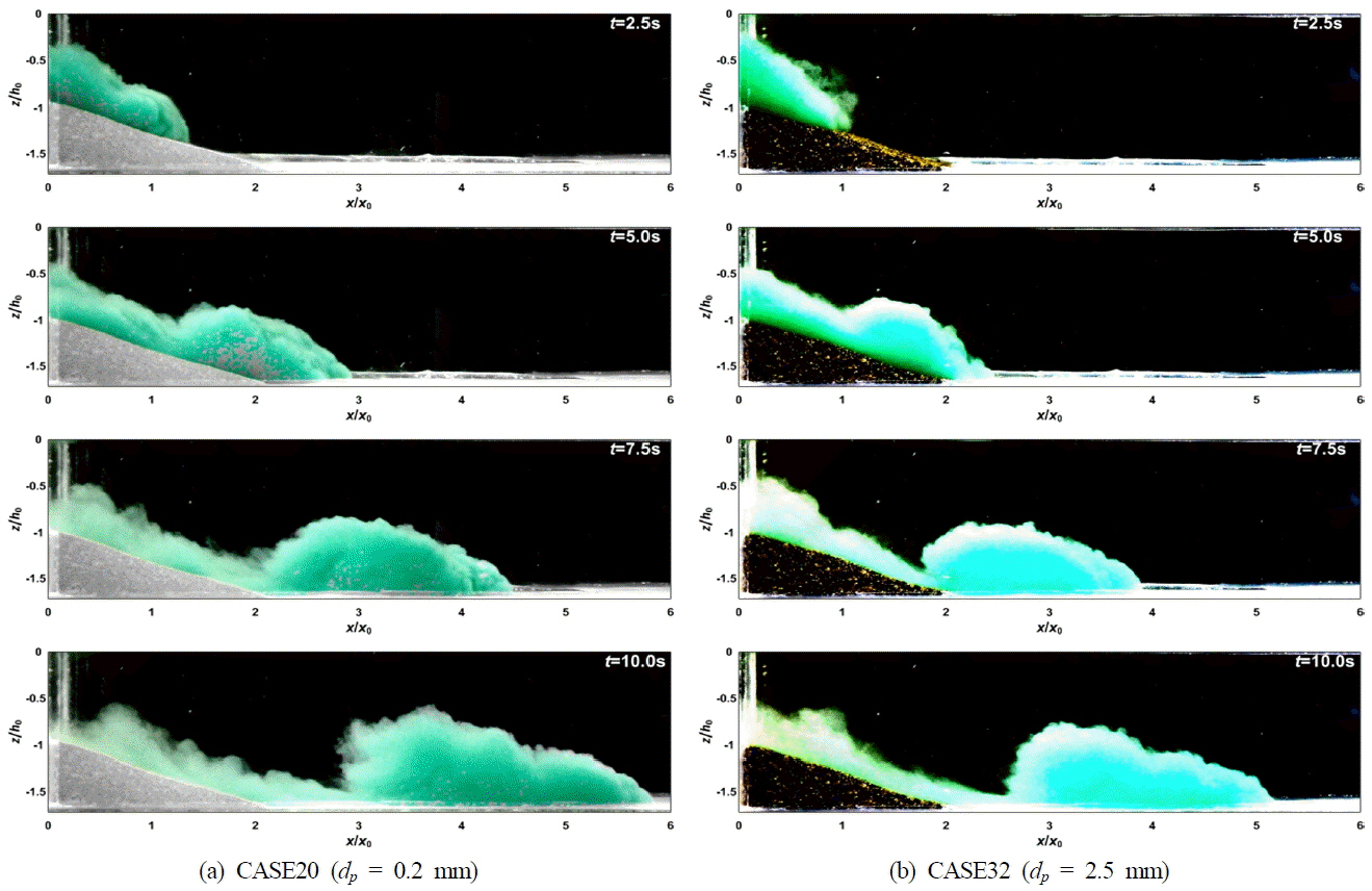
Time series of contour shapes by advection-diffusion of saltwater over permeable sloping bed of 1:3

In Fig. 8, the behavior of advection-diffusion of saltwater has a similar shape with the impermeable bottom condition (Fig. 7), but the spread speed decreases due to the permeable bottom as mentioned in Figs. 6(b) and 6(c). Also, the characteristics according to the diameter of permeable slopping bottom show different head size and shape of saltwater due to the shear force caused by the roughness of slopping bottom and the velocity of saltwater intrusion into a permeable bottom. More detailed study will be available through the experimental results of various permeable bottom conditions, and it is not appropriate to discuss further this issue in this study.

With these results, the difference of spreading characteristics with bottom conditions can be explained through the analysis of flow field and vorticity field obtained with the PIV system, and the influence on advection-diffusion of saltwater is analyzed.

3.2 Flow and Vorticity Field Characteristics on Density Current

In this study, by analyzing the particle track from PIV system using 2-D flow field analysis software (DIPP-FLOW^®), x-z flow components (u and w) are calculated in a unit area of 32 pixel × 32 pixel (1.25 cm × 1.25 cm). The estimated flow velocities are applied to Eq. (1) of Raffel et al.(1998) and Raffel et al.(2007) in order to calculate the vorticity in the x-z plane rotating around y-axis. Here, the clockwise vorticity is expressed in a positive value and the counterclockwise one is expressed in a negative value.

(1) ωx,z=(ΩA+ΩB−ΩC−ΩD)4ΔxΔz

(2) ΩA=12Δx(ui−1,k−1+2ui,k−1+ui+1,k−1)

(3) ΩB=12Δz(wi+1,k−1+2wi+1,k+wi+1,k+1)

(4) ΩC=12Δx(ui+1,k+1+2ui,k+1+ui−1,k+1)

(5) ΩD=12Δz(wi−1,k+1+2wi−1,k+wi−1,k−1)

3.2.1 Characteristics due to Initial Salinity

Fig. 9 shows the flow field and vorticity field according to advectiondiffusion of saltwater in the compartment; Fig. 9(a) is for the initial salinity of 10 psu and Fig. 9(b) is for the initial salinity of 30 psu in the compartment. Given that this is the result when the head of saltwater arrives at x/x₀ 2.5, Fig. 9(a) is t 7.92 sec and Fig. 9(b) is t 4.44 sec. Here, the red corresponds to the clockwise vorticity and the blue corresponds to the counterclockwise one.

Fig. 9.

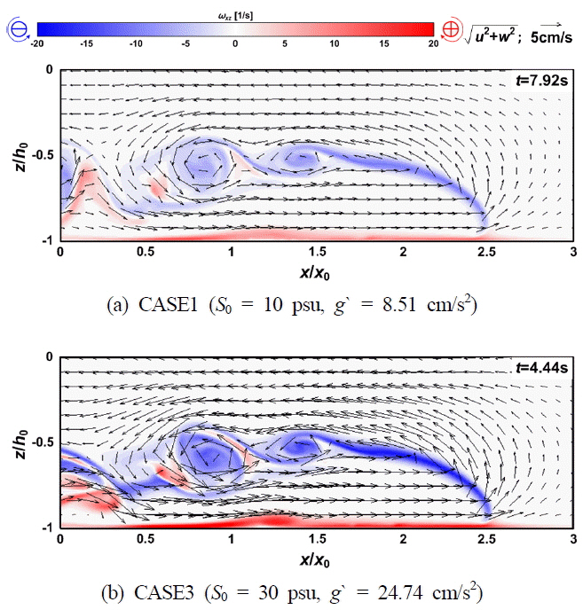
Flow and vorticity field by advection-diffusion of saltwater over impermeable bottom

In Fig. 9, as relatively heavy saltwater proceeds along the bottom, the freshwater moves in the opposite direction in the upper region of flow field by advection-diffusion of saltwater seeping into the freshwater due to the density difference. In Fig. 9(b) CASE3 (g` = 24.74 cm/s²) with higher reduced gravity, the inflow speed of freshwater increases because of the high-speed of saltwater. In addition, Karmann vortex develops along the interface of saltwater and freshwater because of Kelvin-Helmoholtz instability, and there is strong vortex and shedding phenomenon in case of Fig. 9(b) CASE3 (g` = 24.74 cm/s²)with higher spreading rate of saltwater. This phenomenon implies that there is an active saltwater spread.

3.2.2 Characteristics due to Bed Condition

Fig. 10 shows the flow field and vorticity field by advectiondiffusion of saltwater; Fig. 10(a) is the permeable bottom condition of diameter 2.5 mm and Fig. 10(b) is the slopping bottom condition of 1:2. This is the result when the 20 psu saltwater of compartment reaches x/x₀ 2.5; Fig. 10(a) is t 5.75 sec and Fig. 10(b) is t 4.34 sec. Here, the red shows the clockwise vorticity and the blue shows the counterclockwise one. As mentioned above, the spreading rate of saltwater proceeding on the permeable ground by density difference decreases due to the shear stress applied in/out of the surface influenced by the bottom roughness and the saltwater seeping into the ground. In Fig. 10(a), the flow velocity on the bottom decreases and the head shape of saltwater changes, resulting in the distribution of flow field and vorticity field different from the impermeable bottom condition (Fig. 9). Furthermore, because of the decreased spreading rate of saltwater, less vortex shedding can be observed.

Fig. 10.

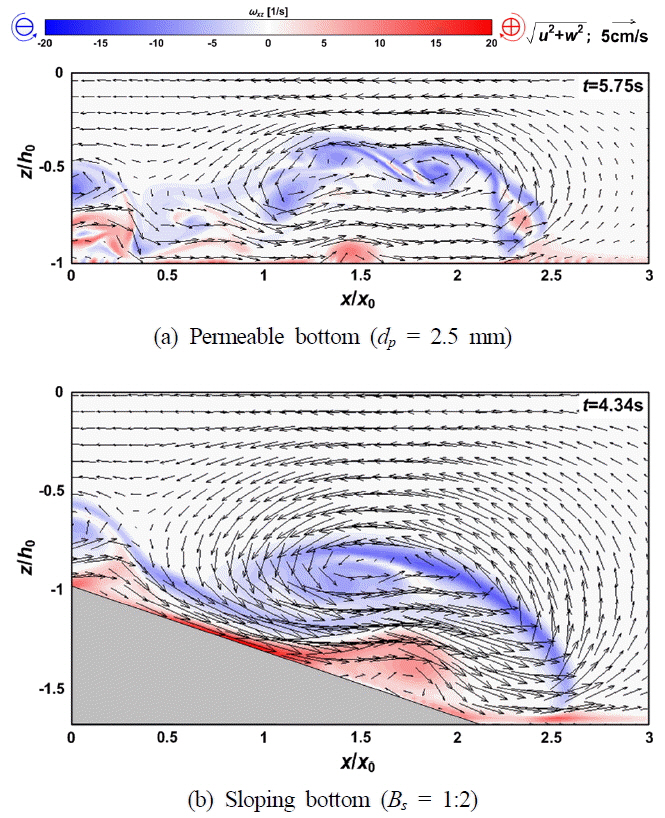
Flow and vorticity field by advection-diffusion of saltwater over permeable and sloping bed

In Fig. 10(b), the flow field and vorticity field show completely different shape from the flat bottom condition. When the saltwater spreads along the slopping bottom, it moves in a mass weakening Kelvin-Helmholtz instability of interface and becomes stable, so Karmann vortex does not develop well.

From the results of flow field and vorticity field, it is found that, when reduced gravity (density difference) increases, spread speed of saltwater increases and shedding of Karmann vortex develops due to the Kelvin-Helmholtz instability in the boundary interface. In addition, different bottom conditions form different flow field and vorticity field. This phenomenon is considered to have great influence on the saltwater spreading on the interface.

3.3 Vertical Distribution of Salinity

Before the discussion of salinity, it is important to mention that this experiment measured vertical distribution of salinity when the pressure was balanced (i.e. all the flow velocities are 0 cm/s). However it is difficult to analyze dependent variable (salinity) according to independent variables such as bottom inclination and bottom permeability. The reason is the fact that it moves along the longer flat bottom until the pressure is balanced after the saltwater passes through slopping bottom, so the effect of slopping bottom cannot be isolated. In addition, when there is a slopping bottom, the distribution area of saltwater becomes different in the water tank, and the saltwater intrusion is excluded when there is a permeable bed. Therefore, this study only handles the characteristics of vertical distribution of salinity for the effect of initial salinity in the compartment.

Fig. 11 shows the vertical salinity distribution normalized by the initial salinity (S₀) according to the initial salinity in a compartment for the impermeable bottom condition, where the salinity is measured at every 1 cm interval from the bottom when there is pressure balance. Here, the black circles (●) are results for the initial salinity of 10 psu (CASE1); the blue squares () are results for the initial salinity of 20 psu (CASE2); and the red diamonds () are results for the initial salinity of 30 psu (CASE3).

Fig. 11.

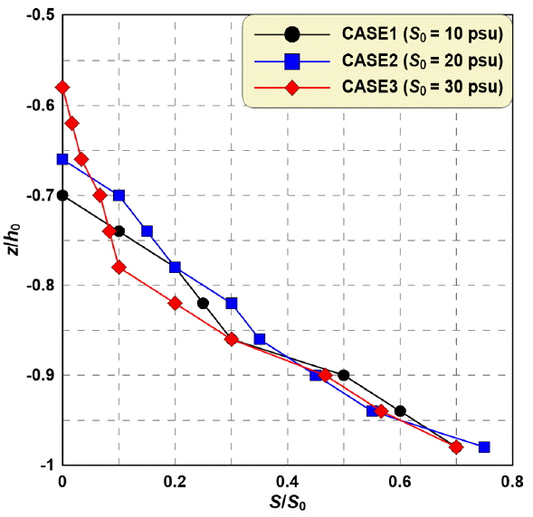
Vertical profile of salinity according to S₀ in still-water

In Fig. 11, the salinity is widely distributed in the vertical direction due to the increased spreading rate of saltwater mass when the S₀ of compartment increases and due to the spread of saltwater by Karmann vortex and vortex shedding at the interface. According to these experimental results, saltwater spread is governed by the vortex and vortex shedding at the interface, and it has great influence on the vertical distribution of salinity.

4. Concluding Remarks

In this study, hydraulic model experiments to which PIV system applied were conducted in order to understand the hydrodynamic characteristics of advection-diffusion of saltwater according to the bottom conditions (impermeable/permeableness, diameter, and inclination) and the differences of initial salinity. Considering the quantitative and qualitative results from the experiment, the characteristics of density current were discussed and they can be summarized as the followings:

(1) The spreading rate of saltwater by advection-diffusion due to the density difference increases as acceleration, which can be described as the reduced gravity, when reduced gravity (g`) increases (density difference increases).

(2) The spreading rate of saltwater due to the advection-diffusion on the impermeable ground decreased due to the bottom roughness and in/out-side shear stress of surface by the saltwater seeping into the ground. In addition, it decreased more when the bed material of permeable bottom was coarse.

(3) In case of advection-diffusion of saltwater falling along the slopping bottom, it moved in a mass so the head develops and it had an oval shape. And it showed relatively stable shape comparing to the flat bottom condition.

(4) Due to the effect of saltwater spreading along the bottom, there is freshwater inflow in the opposite direction on top layer, and this phenomenon becomes stronger when reduced gravity becomes stronger.

(5) Counterclockwise Karmann vortex develops by the Kelvin-Helmholtz instability along the boundary interface of advectiondiffusion saltwater, as well as strong vortex and vortex shedding occur with fast spread speed of saltwater.

(6) The flow velocity of saltwater decreases due to the shear stress formed in/out-side of ground surface and roughness of bottom, and this shows different flow field and vorticity comparing to the impermeable bottom condition.

(7) When the saltwater spreads along slopping bottom, it moves in a mass so that Kelvin-Helmholtz instability of slopping bottom becomes weak and Karmann vortex does not develop so much.

(8) Higher the reduced gravity is (higher the initial salinity of compartment is), faster the saltwater spreads. And Karmann vortex and vortex shedding formed at the boundary interface causes large spreads of saltwater resulting in the vertically wide distribution of salinity.

Acknowledgements

This research was supported by Basic Science Research Program through the National Research Foundation of Korea (NRF) funded by the Ministry of Education (NRF-2015R1D1A4A01020046).

References

Benjamin TB. 1968;Gravity Currents and Related Phenomena. Journal of Fluid Mechanics 31(2):209–248.

Blumberg AF. 1977;Numerical Model of Estuarine Circulation. Journal of Hydraulics Division 103:295–310.

Cantero M, Balachandar S, García M, Ferry J. 2006;Direct Numerical Simulations of Planar and Cylindrical Density Currents. Journal of Applied Mechanics 73(6):923–930.

De Cesare D, Boillat J-L, Schleiss AJ. 2006;Circulation in Stratified Lakes due to Flood-Induced Turbidity Currents. Journal of Environmental Engineering 132(11):1508–1517.

Farhanieh B, Firoozabadi B, Rad M. 2001;The Propagation of Turbulent Density Currents on Sloping Beds. Scientia Iranica 8(2):130–137.

Firoozabadi B, Afshin H, Aram E. 2009;Three-Dimensional Modeling of Density Current in a Straight Channel. Journal of Hydraulic Engineering 135(5):393–402.

Georgoulas AN, Angelidis PB, Panagiotidis TG, Kotsovinos NE. 2010;3D Numerical Modelling of Turbidity Currents. Environmental Fluid Mechanics 10(6):603–635.

Gill AE. 1982. Atmosphere-Ocean Dynamics New York: Academic Press.

Gray TE, Alexander J, Leeder MR. 2006;Longitudinal Flow Evolution and Turbulence Structure of Dynamically Similar, Sustained, Saline Density and Turbidity Currents. Journal of Geophysical Research: Oceans Banner :111.

Hormozi S, Firoozabadi B, Ghasvari H. 2008;Characteristic Variables and Entrainment in 3-D Density Currents. Scientia Iranica 15(5):575–583.

Huppert HE, Simpson JE. 1980;The Slumping of Gravity Currents. Journal of Fluid Mechanics 99(4):785–799.

Lal PBB, Rajaratham N. 1977;Experimental Study of Bluff Buoyant Turbulent Surface Jets. Journal of Hydraulic Research 15(3):261–275.

Lesser GR, Roelvink JA, van Kester JATM, Stelling GS. 2004;Development and Validation of a Three-Dimensional Morphological Model. Coastal Engineering 51(8–9):883–915.

Marmoush YR, Smith AA, Hamblin PF. 1984;Pilot Experiments on Thermal Bar in Lock Exchange Flow. Journal of Energy Engineering 110(3):215–227.

Mueller C, Carbone R. 1987;Dynamics of a Thunderstorm Outflow. Journal of the Atmospheric sciences 44(15):1879–1898.

Natale MD, Vicinanza D. 2001;An Experimental Study of Heated Surface Jet in a Wave Environment. The International Society of Offshore Polar Engineers 11:396–403.

Pacanowski RC, Philander SGH. 1981;Parameterization of Vertical Mixing in Numerical Models of Tropical Oceans. Journal of Physical Oceanography 11:1443–1451.

Paik J, Eghbalzadeh A, Sotiropoulos F. 2009;Three-Dimensional Unsteady RANS Modeling of Discontinuous Gravity Currents in Rectangular Domains. Journal of Hydraulic Engineering 135(6):505–521.

Patterson MD, Simpson JE, Dalziel SB, Nikiforakis N. 2005;Numerical Modelling of Two-Dimensional and Axisymmetric Gravity Currents. International Journal for Numerical Methods in Fluids 47:1221–1227.

Raffel M, Willert CE, Kompenhans J. 1998. Particle Image Velocimetry: a Practical Guide Springer Verlag. Berlin: p. 253.

Raffel M, Willert CE, Wereley ST, Kompenhans J. 2007. Particle Image Velocimetry Springer Verlag. Berlin: p. 448.

Sato T, Tonoki K, Yoshikawa T, Tsuchiya Y. 2006;Numerical and Hydraulic Simulations of the Effect of Density Current Generator in a Semi-Enclosed Tidal Bay. Coastal Engineering 53(1):49–64.

Shanack S. 1960;A Theoretical Current Density Ansatz for the Quiet Day Solar Semi-Diurnal Tidal Mode of Oscillation of the Ionosphere. Journal of Atmospheric and Terrestrial Physics 17(4):337–343.

Simpson JE. 1969;A Comparison between Laboratory and Atmospheric Density Currents. Quarterly Journal of The Royal Meteorological Society 95(406):758–765.

Thomas LP, Marino BM, Linden PF. 1998;Gravity Currents over Porous Substrates. Journal of Fluid Mechanics 366:239–258.

Thomas LP, Marino MB, Linden PF. 2004;Lock-Release Inertial Gravity Currents over a Thick Porous Layer. Journal of Fluid Mechanics 503:299–319.

Wakimoto RM. 1982;The Life Cycle of Thunderstorm Gust Fronts as Viewed with Doppler Radar and Rawinsonde Data. Monthly Weather Review 110:1060–1082.

White BL, Helfrich KR. 2008;Gravity Currents and Internal Waves in a Stratified Fluid. Journal of Fluid Mechanics 616:327–356.

Article information Continued

This is an open access article distributed under the terms of the creative commons attribution non-commercial license (http://creativecommons.org/licenses/by-nc/3.0) which permits unrestricted non-commercial use, distribution, and reproduction in any medium, provided the original work is properly cited.

Table 1.

State of water and bed conditions used for watercolor experiments

CASE	Bed			Water basin					Difference

				Small side (Saltwater)			Large side (Freshwater)

	State	Diameter d_p [mm]	Slope B_s	Salinity S₀ [psu]	Temperature T₀ [°C]	Density ρ₀ [g/cm³]	Temperature T_f [°C]	Density ρ_f [g/cm³]	Salinity ΔS [psu]	Temperature ΔT [°C]	Density Δρ [g/cm³]	Reduced gravity g′ [cm/s²]
1	State	Impermeable			10	15.8	1.0073	17.9	0.9986	10	2.1	0.0087	8.51
2	1:∞			20	16.8	1.0155	17.9	0.9986	20	1.1	0.0168	16.52
3				30	16.4	1.0238	17.9	0.9986	30	1.5	0.0252	24.74

4				10	17.5	1.0070	17.9	0.9986	10	0.4	0.0084	8.26
5	1:0			20	16.5	1.0155	17.8	0.9986	20	1.3	0.0169	16.54
6				30	15.9	1.0239	17.9	0.9986	30	2.0	0.0253	24.79

7				10	17.0	1.0071	17.9	0.9986	10	0.9	0.0085	8.34
8	1:2			20	16.9	1.0154	17.8	0.9986	20	0.9	0.0168	16.49
9				30	16.5	1.0238	17.9	0.9986	30	1.4	0.0252	24.73

10				10	16.7	1.0072	17.8	0.9986	10	1.1	0.0085	8.36
11	1:3			20	16.3	1.0155	17.9	0.9986	20	1.6	0.0169	16.59
12				30	15.5	1.0239	17.8	0.9986	30	2.3	0.0253	24.81

13				10	16.5	1.0072	17.1	0.9988	10	0.6	0.0084	8.27
14	1:5			20	15.4	1.0156	18.0	0.9986	20	2.6	0.0170	16.71
15				30	16.5	1.0238	18.0	0.9986	30	1.5	0.0252	24.75

16	permeable			0.2		10	16.4	1.0072	17.5	0.9987	10	1.1	0.0085	8.35
17					1:∞	20	16.7	1.0155	17.3	0.9987	20	0.6	0.0167	16.43
18						30	16.5	1.0238	17.5	0.9987	30	1.0	0.0251	24.66

19			10		16.5	1.0072	17.8	0.9986	10	1.3	0.0085	8.39
20		1:2	20		17.1	1.0154	17.7	0.9987	20	0.6	0.0168	16.45
21			30		16.4	1.0238	17.7	0.9987	30	1.3	0.0252	24.71

22			10		17.4	1.0071	17.7	0.9987	10	0.3	0.0084	8.24
23		1:3	20		16.4	1.0155	17.8	0.9986	20	1.4	0.0169	16.56
24			30		16.0	1.0239	17.9	0.9986	30	1.9	0.0253	24.78

25			10		16.8	1.0071	17.8	0.9986	10	1.0	0.0085	8.35
26		1:5	20		16.7	1.0155	17.7	0.9987	20	1.0	0.0168	16.50
27			30		16.4	1.0238	17.8	0.9986	30	1.4	0.0252	24.72

28		2.5			10	16.8	1.0071	17.5	0.9987	10	0.7	0.0085	8.30
29			1:∞		20	16.9	1.0154	17.5	0.9987	20	0.6	0.0168	16.44
30				30	16.7	1.0238	17.8	0.9986	30	1.1	0.0252	24.69

31				10	17.0	1.0072	17.5	0.9987	10	0.5	0.0084	8.27
32			1:2	20	16.6	1.0155	17.7	0.9987	20	1.1	0.0168	16.51
33				30	16.6	1.0238	17.9	0.9986	30	1.3	0.0252	24.72

34				10	16.5	1.0072	17.6	0.9987	10	1.1	0.0085	8.36
35			1:3	20	16.9	1.0154	17.9	0.9986	20	1.0	0.0168	16.51
36				30	16.7	1.0238	17.9	0.9986	30	1.2	0.0252	24.71

37				10	17.5	1.0070	17.9	0.9986	10	0.4	0.0084	8.26
38			1:5	20	17.1	1.0154	17.9	0.9986	20	0.8	0.0168	16.49
39				30	16.8	1.0238	17.8	0.9986	30	1.0	0.0252	24.68

Table 2.

State of water and bed conditions used for PIV experiments

CASE	Bed			Water basin					Difference

				Small side (Saltwater)			Large side (Freshwater)

	State	Diameter d_p [mm]	Slope B_s	Salinity S₀ [psu]	Temperature T₀ [°C]	Density ρ₀ [g/cm³]	Temperature T_f [°C]	Density ρ_f [g/cm³]	Salinity ΔS [psu]	Temperature ΔT [°C]	Density Δρ [g/cm³]	Reduced gravity g′ [cm/s²]
1	Impermeable			10	16.5	1.0072	17.4	0.9987	10	0.9	0.0085	8.32
2			1:∞	20	17.1	1.0154	17.8	0.9986	20	0.7	0.0168	16.47
3				30	16.3	1.0238	17.9	0.9986	30	1.6	0.0252	24.75

4				10	16.8	1.0071	17.5	0.9987	10	0.7	0.0085	8.30
5			1:0	20	15.5	1.0156	17.4	0.9987	20	1.9	0.0169	16.59
6				30	16.7	1.0238	17.3	0.9987	30	0.6	0.0251	24.60

7				10	15.3	1.0074	17.7	0.9987	10	2.4	0.0087	8.54
8			1:2	20	16.1	1.0155	17.7	0.9987	20	1.6	0.0169	16.57
9				30	15.8	1.0239	17.6	0.9987	30	1.8	0.0252	24.74

10				10	16.4	1.0072	17.9	0.9986	10	1.5	0.0086	8.43
11			1:3	20	16.0	1.0156	17.8	0.9986	20	1.8	0.0169	16.60
12				30	15.9	1.0239	17.4	0.9987	30	1.5	0.0252	24.70

13				10	15.9	1.0073	17.5	0.9987	10	1.6	0.0086	8.43
14			1:5	20	15.7	1.0156	17.5	0.9987	20	1.8	0.0169	16.58
15				30	16.0	1.0239	17.8	0.9986	30	1.8	0.0252	24.76

16	permeable	0.2		10	16.8	1.0071	17.8	0.9986	10	1.0	0.0085	8.35
17			1:∞	20	16.9	1.0154	17.9	0.9986	20	1.0	0.0168	16.51
18				30	15.9	1.0239	17.2	0.9987	30	1.3	0.0251	24.66

19				10	16.3	1.0072	17.1	0.9988	10	0.8	0.0085	8.30
20			1:2	20	16.8	1.0155	17.2	0.9987	20	0.4	0.0167	16.40
21				30	16.6	1.0238	17.5	0.9987	30	0.9	0.0251	24.65

22				10	17.2	1.0071	17.9	0.9986	10	0.7	0.0085	8.31
23			1:3	20	16.9	1.0154	17.7	0.9987	20	0.8	0.0168	16.48
24				30	17.1	1.0238	17.8	0.9986	30	0.7	0.0251	24.65

25				10	16.9	1.0071	17.7	0.9987	10	0.8	0.0085	8.32
26			1:5	20	17.2	1.0154	17.9	0.9986	20	0.7	0.0168	16.47
27				30	16.5	1.0238	17.3	0.9987	30	0.8	0.0251	24.62

28		2.5		10	16.9	1.0071	17.6	0.9987	10	0.7	0.0085	8.30
29			1:∞	20	16.3	1.0155	17.7	0.9987	20	1.4	0.0169	16.55
30				30	15.7	1.0239	17.8	0.9986	30	2.1	0.0253	24.79

31				10	15.8	1.0073	17.5	0.9987	10	1.7	0.0086	8.44
32			1:2	20	16.7	1.0155	17.8	0.9986	20	1.1	0.0168	16.52
33				30	16.2	1.0239	17.5	0.9987	30	1.3	0.0252	24.67

34				10	16.5	1.0072	18.0	0.9986	10	1.5	0.0086	8.43
35			1:3	20	17.4	1.0154	18.1	0.9986	20	0.7	0.0168	16.48
36				30	16.7	1.0238	18.3	0.9986	30	1.6	0.0253	24.79

37				10	17.2	1.0071	18.4	0.9985	10	1.2	0.0085	8.40
38			1:5	20	17.8	1.0154	18.2	0.9986	20	0.4	0.0168	16.45
39				30	16.4	1.0238	18.1	0.9986	30	0.7	0.0252	24.78