


1. Introduction
Humans have attempted to understand various phenomena that occur in the sea many years ago. However, these phenomena are difficult to elucidate even after several centuries because of complex interactions involving physical, chemical, and biological processes (Dawarakish et al., 2013). Hence, various methods have been formulated through statistical analysis, spectrum analysis, time series analysis, empirical formulas based on mathematical model experiments, and other mathematical and physical analyses. However, the derivation of accurate results is limited owing to the complex interrelationships among numerous parameters in nature (Goldstein et al., 2019).
As we enter the era of the Fourth Industrial Revolution, machine learning (ML) models that identify and predict statistical structures from input and output data using computers to solve numerous engineering problems in the natural world are garnering significant attention. ML, a field of artificial intelligence (AI), is an inductive method that identifies rules through learning using data and results, instead of using a conventional program method that derives results from rules and data. ML techniques can easily solve complex engineering problems and enable the regression analysis of nonlinear relationships. ML demonstrates clear advantages over other conventional regression methods because it adopts a specific algorithm that can learn from the input data and provides accurate results via the output (Salehi and Burgue├▒o, 2018). ML-based predictive models include various algorithms such as neural networks, decision trees, support vector machines (SVM), and gradient boosting (GBR). In coastal engineering, studies based on ML-based algorithms are increasingly conducted to predict wave formation, wave breaking, tidal changes, hydraulic properties around structures, and changes in beach profiles (Deo and Jagdale, 2003; Panizzo and Briganti, 2007; Kankal and Yuksek, 2012).
This paper introduces ML models and reviews various studies that predict significant parameters in coastal engineering such as waves, wave breaking, hydraulic properties around structures, and beach profile changes. This paper focuses on regression analysis studies that involve continuous variables for parameters during the supervised learning of ML models, whereas studies pertaining to classification involving categorical variables are omitted. Furthermore, the basic concepts and basic contents of various ML models are introduced, and the technological trends and application examples of ML models in the coastal engineering field are described.
2. Machine Learning Model
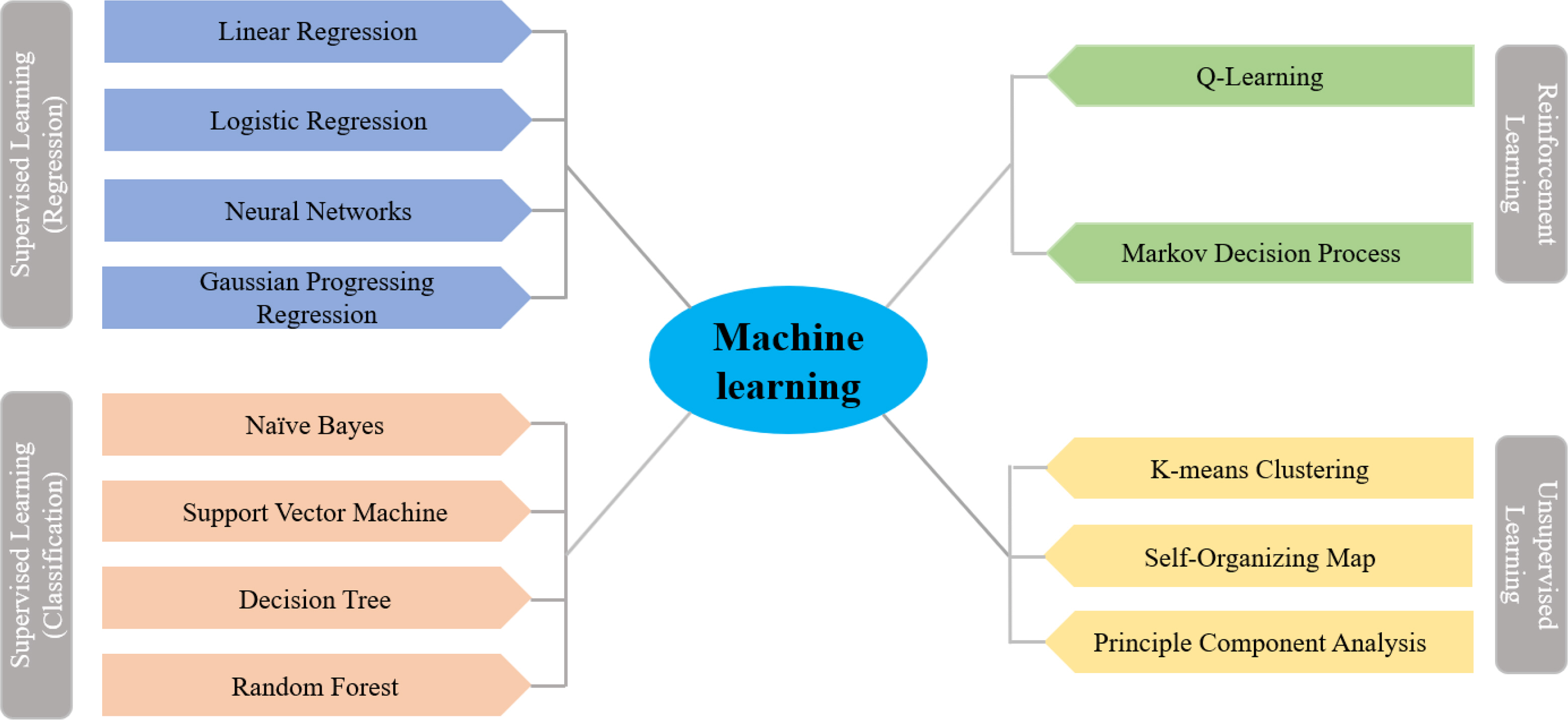
As we enter the era of the Fourth Industrial Revolution, interest in AI and ML is increasing. ML, which is a field of AI, trains computers human thinking and cognition methods such that the computers can perform recognition and inference on their own without preset judgment criteria for all variables. General ML algorithms include supervised learning, unsupervised learning, and reinforcement learning (Fig. 1). Two supervised learning models exist: regression and classification. Data classification and prediction are determined based on the characteristics of both the input and dependent variables. Representative supervised learning algorithms include artificial neural network (ANN), SVM, and random forest (RF). Unsupervised learning is a method of predicting results for new data by clustering patterns or features from unlabeled data. It is primarily used for clustering and dimensionality reduction, e.g., k-means clustering and principal component analysis. This paper focuses on the application cases of coastal and marine engineering for supervised learning among ML algorithms.
2.1 Linear Regression (LR) Model
The LR model uses linear parameters and offers easy and quick analyses. The LR model was developed more than a century ago and has been widely used over the past few decades. However, it yields low accuracy results for data that exhibit nonlinear relationships. LR generates a regression model using one or more features and obtains parameters w and b that minimize the mean squared error (MSE) between the experimental value (y) and predicted value (┼Ę) (Eqs. (1)ŌĆō(2)).
2.1.1 Lasso regression
In some cases, the conventional LR method results in overfitting, i.e., the predictive performance is unsatisfactory when new data are provided. Hence, lasso regression was developed, which limits models by force using the L1 regulation, as follows (Eq. (3)):
where m is the number of weights, and ╬▒ is the penalty parameter. This obtains w and b that minimize the sum of the MSE and penalty.
2.1.2 Ridge regression
Ridge regression is a model in which the L2 regulation term is added to solve the overfitting problem of the LR model. This model not only fits the data of the learning algorithm, but also ensures that the weights of the model are minimized (Eq. (4)).
The difference between lasso regression and ridge regression is that the weights are zero in lasso, whereas in ridge, the weights are approximately zero but not exactly zero. Hence, the lasso regression offers high accuracy only if some of the input variables are important, whereas the accuracy of the ridge model will be high if the importance of the input variables is similar in general.
2.2 ANN
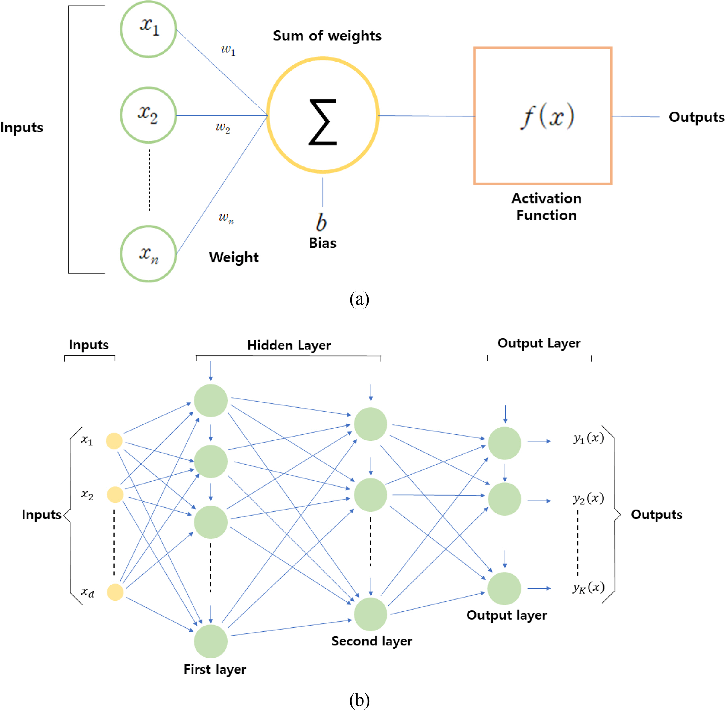
An ANN is an information processing structure in the form of a network modeled based on the human nervous system, where simple functional processors are interconnected on a large scale. The perceptron, which is the basis of deep learning, is a structure designed to deliver information based on a threshold by issuing a weighting signal for input values through the imitation of neuron behaviors in brain cells. Fig. 2 shows the structure of a neural network. A neural network comprises an input layer, a hidden layer, and an output layer, and its nodes are interconnected by weights. In an ANN, the values are transmitted from the input layer to all nodes of the hidden layer in a feedforward method. Moreover, the output values of all nodes of the hidden layer are transmitted to all nodes via the coupling and activation functions. Learning proceeds by redistributing weights between neurons through the backpropagation algorithm such that they converge in a direction in which the errors are reduced to minimize the difference between the predicted and experimental values.
In the data processing process of the neural network, each node multiplies the input value by a weight and then passes the output value through the activation function to the next node to output the result, as expressed in Eq. (5).
where w is the weight, ╬Ė the bias, and x the input value.
The activation function renders the neural network nonlinear and enables a nonlinear analysis of the result calculated from the coupling function via the calculation of the activation function, which is a nonlinear function. Furthermore, the activation function is key for adjusting the gradient during activation training. Various activation functions are used in neural networks, including the linear, sigmoid, tanh, exponential, softmax, rectified linear unit (ReLU), ELU (Exponential Linear Unit), and SELU(Scaled Exponential Linear Unit) functions.
2.3 SVM
The SVM was introduced by Boser et al. (1992), who were inspired by the concept of statistical learning theory. SVM regression performs training to include the maximum amount of data within the specified margin error limit line. The limit line adjusts the width of the margin based on the hyperparameter. Here, the margin implies the distance between the grain boundary and support vector. The procedure of applying the SVM to the regression problem is as follows (Eqs. (6)ŌĆō(7)). First, the dataset for training is distinguished.
where x is the input variable, y the output variable, Rn the n-dimensional vector space, and r the one-dimensional vector space.
The loss function of ╬ĄŌłłsensitive can be expressed as follows:
Based on the above, if the predicted value is within the expected range, then the loss function is 0; if the predicted value is outside the expected range, then the loss function of ╬ĄŌłłsensitive is defined such that the loss is equal to the absolute value of the standard deviation minus ╬Ą. The main purpose of the vector machine is to provide the deviation of ╬Ą in the actual output value and to obtain a uniform function f(x).
Finally, f(x) can be expressed as follows (Eqs. (8)ŌĆō(9)):
where ╬▒i and
╬▒ i *
2.4 Gaussian Process Regression (GPR)
The Gaussian process regression (GPR) model is a probability model based on nonparameteric kernels. The Gaussian process f(x) is a set of random variables f(x) in the range of {(xi, yi); xi ŌłłRd}, where a finite number of randomly selected variables, f(x1), ..., f(xm), among them exhibits a combined Gaussian density (Na et al., 2017). The GPR model for the new input vector (xŌēĀw) and training data predicts yŌēĀw. The linear regression model is expressed as follows:
where ╬Ą Ōł╝N (0, Žā2), and the error variance (Žā2) and coefficient (╬▓) are calculated based on data. The GPR model describes predictions by introducing potential variables in the Gaussian process f(xi ), i = 1, 2,..., n and the explicit basic function h(x). The covariance function of the hidden variable provides flexibility to the response, and the basic function transmits the input of x to the p-dimensional feature space. The Gaussian process is a random variable set that comprises a finite number of Gauss distributions. If {f(x), xi ŌłłRd} is a Gaussian process and n contains the observed values x1, x2,..., xn, then the random variables f(x1),f(x2),..., f(xn ) exhibits a Gaussian distribution. The Gaussian process is defined by the mean function (m(x)) and covariance function (k(x,xŌĆ▓)).
Here, h(x) is a basic function set that transmits the existing feature vector x of Rd to the new feature vector h(x).
Therefore, the GPR model can be represented as a probabilistic model as in Eq. (15), and the hidden variable f(xi ) is introduced to observe each xi (Koo et al., 2016).
2.5 Ensemble Method
The ensemble method is developed to improve the performance of the classification and regression tree. It generates an accurate prediction model by creating several classifiers and combining their predictions. In other words, it is a method of deriving a high-accuracy prediction model by combining several weak classifier models, instead of using a single strong model.
The ensemble models can be primarily categorized into bagging and boosting models. Bagging is a method of reducing variance using the averaging or voting method on the results predicted using various models, whereas boosting is a method of creating strong classifiers by combining weak classifiers.
2.5.1 RF
RF is a method of improving the large variance of the decision tree and the large performance fluctuation range. It combines the concept and properties of bagging with randomized node optimization to overcome the disadvantages of existing decision trees and improves generalization. The process of extracting bootstrap samples and generating a decision tree for each bootstrap sample is similar to bagging. However, it is different from the conventional decision tree in that a method of randomly extracting predictors and creating an optimal split within the extracted variables is used instead of selecting the optimal split within all predictors for each node (Kim et al., 2020). In other words, RF combines the randomization of predictors while determining slightly different training data through bootstrap to obtain maximum randomness. Hence, several low-importance learners are created. The important hyperparameters used in an RF include max_features, bootstrap, and n_estimator. The max_features parameter refers to the maximum number of features to be used in each node. The bootstrap allows redundancy in data sampling conditions for each classification model. The n_estimator refers to the number of trees to be created in the model (Kim and Kim, 2020).
2.5.2 Boosting method
Boosting is a technique for creating a strong classifier from a few weak classifiers. It is a model created by boosting weights on data at the boundary. The adaptive boosting (AdaBoost) algorithm is the most typically and widely used algorithm among ensemble learning methods. Specifically, it is one of the boosting series in ensemble learning. In AdaBoost, after a weak classifier is generated using the initial training data, the distribution of the training data is adjusted based on the prediction performance afforded by the training of the weak classifier. The weight of the training sample with low prediction accuracy is increased using the information received from the classifier in the previous stage. In other words, the training accuracy is improved by adaptively changing the weights of samples with low prediction accuracy in the previous classifier. Finally, a strong classifier with slightly better performance is created by combining these weak classifiers with low prediction performance. GBR is a method of sequentially adding multiple models such as the AdaBoost model. The most significant difference between the two algorithms is the method by which they recognize weak classifiers. AdaBoost recognizes values that are more difficult to classify by weighting them. By contrast, GBR uses a loss function to classify errors. In other words, the loss function is an index that can evaluate the performance of the model in learning specific data, and the model result can be interpreted based on the loss function used.
AdaBoost can be used for both classification and regression. In general, when a regression problem is considered, the training data set can be expressed as follows:
where (Xi, Yi)(i = 1,...,m) is the ith sample of the training dataset, m the total number of samples, Xi the input data vector value, and Yi the output data value.
Next, we can train a weak classifier G(X) using a specific learning algorithm, and the relative prediction error ei of each sample is expressed as follows:
where L(ŌłÖ) is the loss function. In general, three options are available: linear loss, square loss, and exponential loss. For a simple explanation, the linear loss is applied as follows:
where E = max|Yi ŌłÆ G(Xi)|is the maximum absolute error of all samples.
The performance of one weak classifier will inevitably be unsatisfactory. Hence, the objective of AdaBoost is to sequentially generate weak classifiers Gk (X), k = 1,2,...,N, and then combine them. A strong classifier H(X) is composed of a few combination strategies. For regression analysis, the combination is expressed as follows:
where ak is the weight of the weak classifier (Gk (X)), g(X) is the median of all akGk (X), k = 1,2,...,N, and ╬ĮŌłł[0,1] is used as a regulatory factor or to prevent overfitting. Both the weak classifier (Gk (X )) and weight ak are generated using the modified value of the existing learning data. As such, the distribution weight of each sample is adjusted based on the error predicted by the previous weak classifier (GkŌłÆ 1 (X)). Incorrectly predicted samples are repeatedly trained by increasing the weight such that they will be prioritized in the next learning process. During the iteration of k = 1,2,...,N, the weak classifier (Gk (X )) and relative prediction error eki are calculated using Eq. (19). Subsequently, the total error rate ek is expressed as follows (Eq. (20)):
Furthermore, the weight ak of the weak classifier can be represented as follows (Eq. (21)):
Finally, for the next step learning, the weight distribution of each sample (wk+ 1,i) is updated again as follows (Eq. (22)):
Between the two types of weights (wk, ╬▒k) defined above, the first (wk) involves training the data sample and is used to enable better training in the next step after the weight of the incorrectly predicted sample is increased. The second (╬▒k) implies a weak classifier and is used to such that a more accurate weak classification will impose a greater effect on the final result. AdaBoost provides a stronger framework than specific learning algorithms because it does not provide a specific form of the weak classifier G(X). Theoretically, every type of ML regression algorithm can be used as a weak classifier in AdaBoost.
3. Application of ML in Coastal and Marine Engineering Field
3.1 Wave Prediction
Accurate wave estimations can be applied to coastal engineering, marine transportation, and leisure sports. For example, the transportation route can be optimized by reducing the transportation time through accurate wave information prediction, which can provide accurate prediction information regarding the generation of wave energy. Furthermore, useful information can be provided to surfers in a surf zone by providing wave information at a coast. Significant wave height is an important parameter in coastal port structure design and construction. Most physics-based models are applied to estimate such wave information. However, wave estimation studies based on ML models have increased recently (Deo and Naidu, 1999; Balas et al., 2004; Mahjoobi et al., 2008; Shahabi et al., 2016; Oh and Suh, 2018; Garcia et al., 2021).
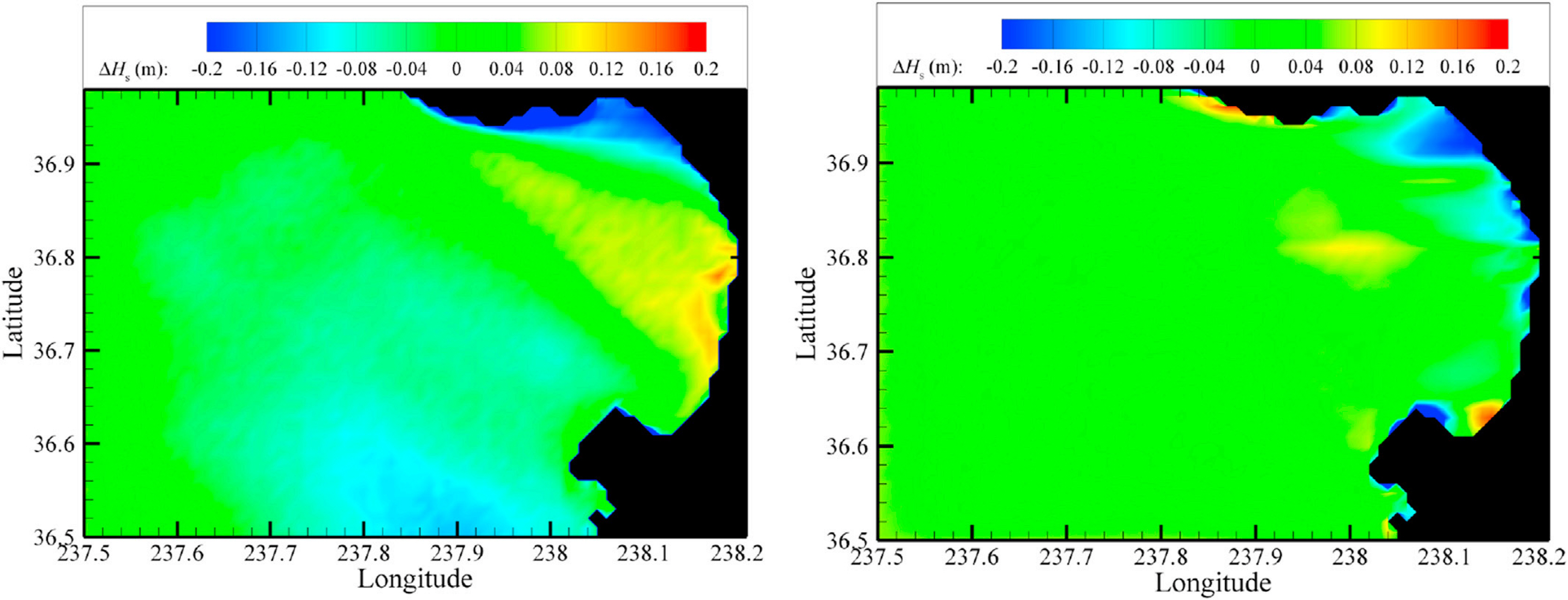
James et al. (2018) developed an ML model to predict the characteristics of wave distributions. Data were generated via a few thousand rounds of iterative learning using a physics-based model known as the simulating waves nearshore (SWAN) model. Furthermore, a model for predicting the significant wave height and peak period using a multilayer perceptron and an SVM was proposed. A total of 741 input variables were applied considering the wave conditions at the interface (Hs, Ts, D), flow distribution within the grid (u,v), wind speed, and wind direction. Meanwhile, 11,078 data points were used for training, where two output variables (i.e., the significant wave height and peak period) calculated using the SWAN model were applied (Table A1). The result shows that the ML model reproduced more than 90% of the wave characteristics of the physics-based model, with an MSE of 9 cm. Moreover, the computation time is shorter compared with that afforded by the SWAN model; therefore, it is expected to be a promising alternative to the physics-based model. Fig. 3 shows a heat map presenting the difference (ΔH) between the value predicted by the representative ML model and the value calculated using the SWAN model for the result of the ML model based on data derived from the calculations of 11,078 cases using the SWAN model. The image on the left shows the result of underestimating the significant wave height to a maximum of 15 cm near the bay, although the RMSE is 6 cm. However, the image on the right indicates an RMSE of 14 cm, although the error near the bay is smaller, and a clear location-based trend is not shown. Although statistical values such as the RMSE are important, the reliability of the model may differ by the application purpose. Therefore, the accuracy should be further improved through additional data analysis.
Shamshirband et al. (2020) constructed three ML models, i.e., the ANN, support vector regression (SVR), and the extreme learning machine (ELM) for wave height estimation and compared their performances with the results of the SWAN model. The input variable applied to the ML models was the near-surface wind speed, and the output variable was the significant wave height measured at the Bushehr and Assulayeh Ports of the Persian Bay. These variables were applied to training. The prediction performance of the ELM model was excellent, and the ML-based model of the Bushehr Port was reliable. However, for the Assaluyeh Port, the prediction accuracy for the significant wave height was low, and a correction was performed to improve the efficiency. Furthermore, the result of the ML model underestimated the extreme values. Hence, accurate input values and data preprocessing technology are necessitated to improve the result. The results of the SWAN model underestimated the extreme wave height. Both models require improvement for predicting extreme wave conditions. The ML-based model can be implemented at a low computational cost without requiring the depth information. However, unlike the SWAN model, it requires a separate model to predict the wave height of locations other than the two points used for training.
Chen et al. (2021) proposed a new surrogate model developed using the RF method, which is an ML model, based on spatial wave data estimated using the SWAN numerical model. Twelve input variables were used for model training: the significant wave height (Hs), mean wave direction (mDir), period (Tz), and peak period (Tp) at three buoys. For the output variable, the spatial wave information derived via SWAN calculation was used. The result of the ML model agreed better with the on-site buoy observation values than with the result of the SWAN model, and the computation time of the ML model was 100 times shorter than that of the SWAN model.
Kim et al. (2010) calculated the expected damage of an inclined breakwater using an ANN. The ANN, which uses the tide level and deep-sea waves as input, was trained to predict shallow-sea significant waves. They proved that a high degree of expected damage can be estimated within a short duration by calculating the shallow sea waves.
Kang and Oh (2019) investigated the prediction of swell wave generation using the RF, logistic regression, the K-nearest neighbor algorithm, the ANN, and the SVM. Changes in the water temperature, atmospheric pressure, and tide level were confirmed as primary variables for predicting swell high waves. Furthermore, the RF model performed the best (prediction accuracy: 88.6%).
Park et al. (2020) estimated the significant wave height of an X-band radar using an ANN; this method was demonstrated to be superior over the conventional wave height observation method. The result of a comparative analysis based on Hujeong Beach in Uljin confirmed the high accuracy of the calculated significant wave height.
Lee et al. (2020) conducted a wave breaking prediction study using an open-source ML algorithm to quantitatively predict wave breaking on a coast. The prediction results for the wave breaking wave height and depth by their trained neural network showed better prediction performance compared with the results calculated using the conventional empirical formula.
3.2 Tide Level Prediction
Accurate predictions of the tide level are crucial because the tide level significantly affects navigation, leisure activities, and coastal ecosystems. Tides refer to the periodic ascent and descent of the EarthŌĆÖs sea level due to tidal forces caused by the sun and moon. Thus, the tide level is an important parameter in terms of coastal engineering, maritime safety, and maritime activities. Various other factors such as the wind speed and atmospheric pressure must be considered in addition to the tide level. A harmonic analysis method in which many sine wave components are superimposed is generally used to predict the tide level; however, the effects of time-dependent factors are difficult to consider in this method. This paper introduces research cases that apply an ML model for tide level prediction in coastal and marine engineering.
The conventional harmonic decomposition method requires a significant amount of observational tidal data. Moreover, the parameters of the harmonic analysis model are estimated using the least-squares method based on data obtained for a long duration (i.e., more than 1 month). Lee (2004) constructed an ANN model using short-term measurements for tide level prediction and applied the cos (wntj) and sin (wntj) functions for 69 tidal components as input variables. Consequently, the primary components were determined based on two monthsŌĆÖ worth of measurement data. A comparison between the ANN and harmonic analysis models showed improved accuracy by the ANN model. Moreover, when 15 d of observation data were applied to training, the model presented prediction results that were applicable for predicting the tide levels for 1 year.
These tidal changes involve complex processes that are affected by not only the movement of celestial bodies, but also by nonperiodic meteorological factors such as wind, atmospheric pressure, and water temperature. However, the effect of time-dependent factors cannot be considered using the conventional harmonic analysis method. Therefore, Li et al. (2018) developed a tide level prediction model using the ELM to consider various nonlinear factors such as wind, air pressure, and water temperature. They presented results with higher accuracy and time efficiency than those yielded by conventional harmonic analysis models.
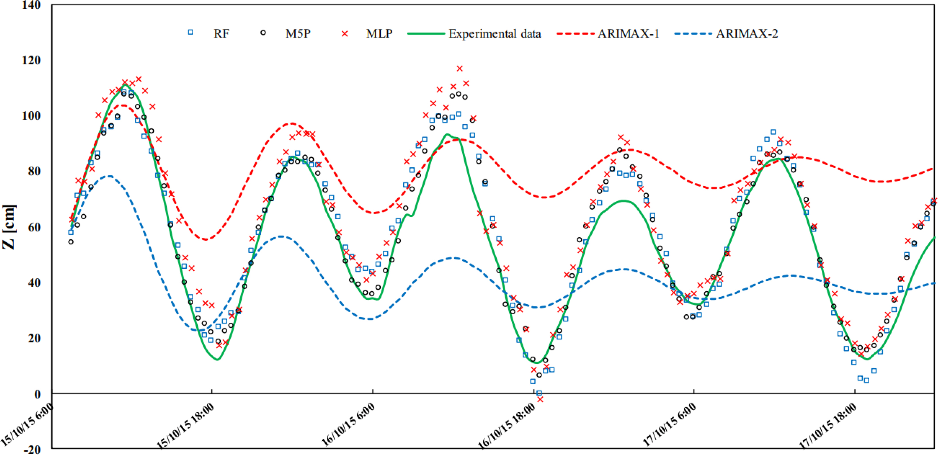
Granta and Nunno (2021) suggested a tide level prediction model using M5P, RF, and ANN algorithms (which are ML models). A total of 28 input variables were used in that study, including the astronomical tide (AT), wind speed (WS), barometric pressure (BP), and previously observed tide levels (ZŌłÆ24 to ZŌłÆ1) to construct a tide level prediction model. Fig. 4 shows the tide level prediction results using the three ML models and the ARIMAX regression analysis. The M5P model showed a high coefficient of determination of 0.924ŌĆō0.996. The result of sensitivity analysis showed high-level prediction results without considering meteorological factors (WS, BP), including for exceptionally high water levels. These results suggest that the training dataset can be continuously updated and applied to sea level fluctuations caused by climate change and subsidence.
3.3 Estimation of Design Variables
Several phenomena pertaining to waveŌĆōstructure interactions exist, such as reflections in the structure, wave breaking on the slope and at the front, dissipation, wave runups and rundowns, transmitted waves, and overtopping. Therefore, techniques for understanding and quantitatively estimating these phenomena are required for the design of structures. Various studies have been conducted to estimate the primary design variables (Goyal et al., 2014; Lee and Suh, 2019; Lee and Suh, 2020; Etemad-Shahidi et al., 2016; Najafzadeh et al., 2014). Herein, we provide examples of applying the ML model for calculating the stability number, overtopping rate, wave transmission coefficient, and reflection coefficient.
3.3.1 Estimating stability number
Kim and Park (2005) constructed a stability number calculation model for rubble-mound breakwater using an ANN. For the input variables of the model, seven parameters were applied, including porosity (P), the number of wave attacks (NW), damage level (Sd), structure slope (cos╬▒), wave height (Hs), wave period (Ts), dimensionless water depth (h/Hs ), and spectral shape (SS). Moreover, the stability number (Ns) was set as the output model. The result shows that the ML model demonstrated higher accuracy in predicting the stability number and damage level compared with the results obtained using the conventional empirical formula. Therefore, it can be utilized for design purposes.
Yagci et al. (2005) modeled the damage rates of different breakwaters using ANN, multiple LR, and fuzzy models. The experimental results yielded by the multiple LR model were unsatisfactory. However, they reported that the neural network and fuzzy model results can be estimated through interpolation for missing values.
EtemadŌĆōShahidi and Bonakdar (2009) constructed a stability prediction model for rubble-mound breakwater using the MŌĆÖ5 model. Five input parameters were applied to the model: porosity (P), the number of wave attacks (NW), damage level (Sd), surf similarity coefficient (╬Šm), and dimensionless water depth (h/Hs). Based on comparison, the results obtained showed higher accuracy compared with those obtained using the conventional Van der Meer empirical equation. A new was derived based on the M5ŌĆÖ model, which proved to be useful for engineering design.
Based on the experimental data of Van der Meer et al. (1988), Koc et al. (2016) suggested a stability number prediction model for breakwater using the genetic algorithm. The experiment result showed that the genetic algorithm afforded better prediction performance than the empirical for the stability number.
3.3.2 Estimating overtopping rate
EurOtop is a representative result of a study that predicted the overtopping rate using an ML tool. In the Crest Level Assessment of Coastal structures by Full-scale Monitoring, Neural Network Prediction, and Hazard Analysis on Permissible Wave Overtopping (CLASH) project (De Rouck et al., 2004), an ANN model was developed to predict the mean overtopping rate, q (Pullen, 2007).
Van Gent et al. (2007) constructed an ANN-based prediction model to estimate the overtopping rates of various coastal structures. A database comprising approximately 10,000 mathematical model data points obtained from the European CLASH project was used for model training. A complexity factor and a reliable factor (RF) were introduced to increase data reliability. Data with low reliability or high complexity were excluded from training. Subsequently, the remaining data were converted to Hm0,toe = 1 m by applying FroudeŌĆÖs law of similarity to match with the mathematical model test results. Fig. 5 describes the parameters used for training. As input variables, 15 parameters describing wave characteristics (e.g., the significant wave height, average period, and wave direction) and factors pertaining to the structural shape (e.g., ridge depth, crest width, and slope) were applied. The mean overtopping rate (q) was set as a dependent variable. The result suggests that the ANN model is sufficiently applicable for modeling the correlation between the input variables related to overtopping and the average overtopping rate in coastal structures. However, all datasets were applied for training without segmenting the dataset in this study, and data with q < 10ŌłÆ6 m3/s/m were excluded from training. Therefore, the generalization of the model is likely to be difficult.
Subsequently, errors in the CLASH database were corrected, and more than 17,000 datasets were expanded through the Innovative Technologies for Safer European Coasts in a Changing Climate project (Zanuttigh et al., 2014). The calculation for the overtopping rate and the estimated results for uncertainty were presented using an ANN model. In previous studies, data with q < 10ŌłÆ6 m3/s/m were removed as measurement errors by experiment were assumed to have increased. However, Zanuttigh et al. (2016) categorized all data into three quantitative classifiers and constructed a training and a prediction model. The result showed improved prediction accuracy compared with the results of previous studies, and the generalization performance was high even for data not used for training.
Den Bieman et al. (2020) and Den Bieman et al. (2021) constructed an overtopping rate prediction model using extreme gradient boosting (XGBoost)ŌĆöan ML model. The result shows that the prediction error was 2.8 times lower than that of the existing neural network model. Moreover, they conducted variable importance analysis via feature engineering. The result shows that the XGBoost model can be successfully applied as an alternative to the ANN model.
Hosseinzadeh et al. (2021) constructed a mean overtopping rate prediction model for an inclined breakwater using GPR and SVR models, which are two kernel-based ML models. The result showed that the accuracy of the GPR model was higher than that of the conventional ANN model and empirical formula. Furthermore, they derived an optimal combination of input variables through sensitivity analysis and demonstrated that the prediction yielded is more accurate than that afforded by the combination of input variables by Van der Meer et al. (2018).
3.3.3 Wave trasmission and reflection coefficients
Formentin et al. (2017) proposed a prediction model for the mean overtopping rate and wave transmission/reflection coefficients (Kt and Kr) using the CLASH database to predict waveŌĆōstructure interactions. An ANN was applied (as an ML model), and 15 nondimensional input variables were applied while considering the structural characteristics (geometric structure, amplitude, and roughness) and wave attack (wave slope and wave direction). Moreover, the overtopping rate, wave transmission coefficient, and reflection coefficient were set as output variables. The result showed that the ANN model afforded a higher prediction accuracy than the existing empirical formula and can be useful for design.
Kuntoji et al. (2018) proposed a prediction model for the wave transmission rate of underwater breakwaters using SVM and ANN models. They developed a model by applying eight input variables, including the wave slope (Hi/gT2) and relative reef width. The prediction result showed that the SVM model to which the kernel function was applied afforded a higher accuracy than the ANN model with an coefficient of dtermination (R2) value of 0.984.
Gandomi et al. (2020) estimated the wave transmission and reflection coefficients of permeable breakwater structures using a genetic algorithm, an ANN, and an SVM. Seven input variables including the porosity, relative wave height, and wave slope were applied as input variables. Moreover, the wave transmission and reflection coefficients were set as output variables. The result showed that the exponential GPR model performed the best for a correlation analysis between experimental and predicted values. They proposed a formula for calculating wave transmission and reflection coefficients using a Gaussian model.
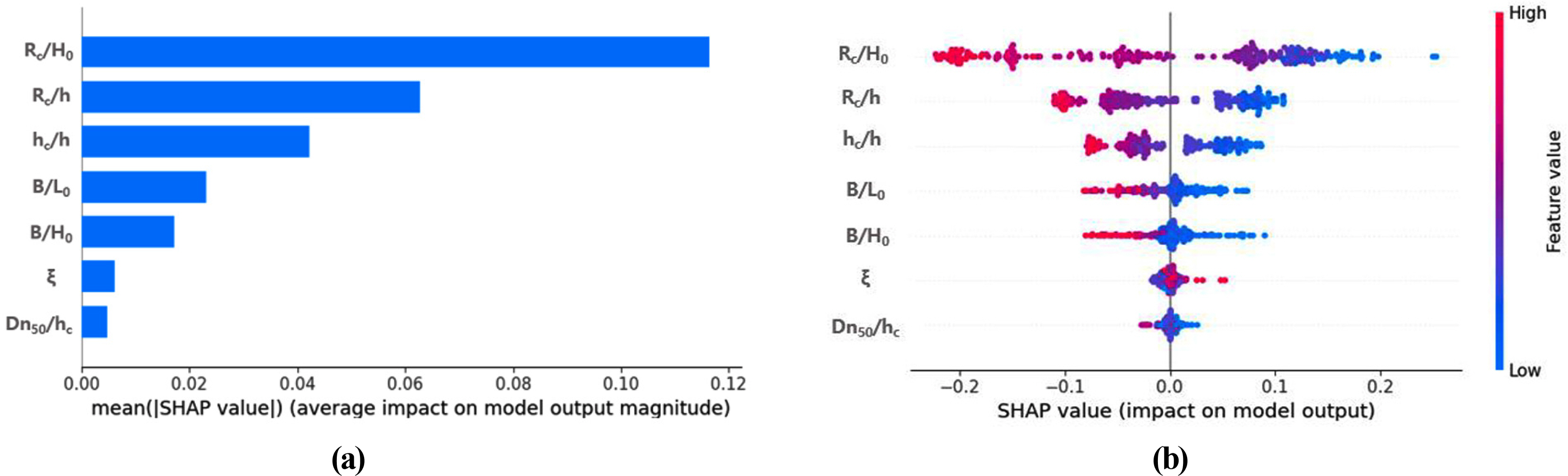
Kim et al. (2021) constructed an ML model for estimating the wave transmission coefficient of low-crested structures using data from a mathematical model used in an experiment conducted through the DELOS project. They adjusted the hyperparameters via grid search for 10 ML models such as GBR, AdaBoost, and Gaussian regression, and selected an ML model suitable for the data. Seven nondimensional input variables such as the relative ridge depth and relative crest width were applied as input variables, whereas the wave transmission coefficient was set as an output variable. In addition, they analyzed the correlation between the input variable and the dependent variable using an explanatory AI technique and determined the dominant factor affecting the prediction of the wave transmission coefficient. Fig. 6 shows the variable importance results for each input variable based on the dependent variable analyzed using the ML analysis tool. The factor related to the ridge depth contributed the most toward the prediction of the output variable. This suggests that the reliability of the model should be improved through model analysis instead of constructing a simple ML model.
3.4 Prediction of Morphological Changes
Studies for further understanding and predicting shoreline fluctuations have been actively conducted, owing to the possibility of increasing coastal erosion acceleration promoted by climate change over the past few decades. The quantitative prediction of coastal erosion and restoration is effective for mitigating erosion risks and is essential for establishing a strategic beach management plan. Therefore, the prediction of beach profile deformation due to waves and beach currents is one of the most important tasks in coastal engineering. Various factors such as wind and waves, beach slope, tide level, sediment particle size, and storm surge frequency can affect beach deformation. Various approaches are available for predicting changes in the beach profile. Sediment movement, erosion, and deposition along a coast are primarily estimated based on empirical formulas; however, the corresponding physical mechanism has not been fully clarified. Recently, data-based ML models have been introduced and used for predicting shoreline fluctuations, barrier islands, and sand dune erosion (Yoon et al., 2013; Wilson et al., 2015; Passarella et al., 2018).
Hashemi et al. (2010) predicted the seasonal variation characteristics of beach profiles using an ANN model based on seven yearsŌĆÖ worth of beach profile data from 19 stations near Tremadoc Bay. Nine parameters were applied as input variables for the model, i.e., the minimum wind speed, wind direction, continuous storm frequency, storm frequency, significant wave height, significant period, wave, beach slope, and wind duration. In addition, they constructed a model using 12 output variables, i.e., the elevation of 10 points of each cross-sectional profile, the area under each profile curve, and the length of the profile. The result showed that the MSE converged to 0.0007 compared with the observed value, demonstrating the high prediction accuracy of the model in estimating beach variability characteristics. These study results suggest that the ML model can be a more effective tool for predicting changes in the beach profile than the mathematical model for the same points, owing to the complexity and uncertainty associated with the physical understanding of morphological dynamics at the shore. However, the ML model is applicable to only previous measurement data; it cannot be applied easily to abnormal climates or structures that are not reflected in the training data. Therefore, a study combining mathematical models and ML is necessary.
Rigos et al. (2016) constructed a model comprising an ANN using the feedforward method to predict the beach circulation pattern of a coast comprising a reef. The beachrock reef in front of the beach increased the complexity of wave actions and nonlinearities. Legendre polynomials were applied as an activation function to reflect this nonlinearity. Data for training were obtained from long-term time-series data for 10 months from January to November 2014 on the target coast. Six independent variables were applied as input variables, i.e., the ridge depth, structure slopes, structure width, significant wave height, and peak wave period. Subsequently, the model was built by setting the offshore distance as a dependent variable.
L├│pez et al. (2017) predicted the sandbar generated on a coast by applying an ANN model. Seven input variables were applied, including the wave characteristics, sediment characteristics, and time data. A model was constructed to predict the location of the sandbar crossing the shore based on six dependent variables at the barrier islandsŌĆÖ feature points (start, ridge, and end points). The results showed that the error of the neural network model was lower than that of the general empirical formula for predicting the characteristics of barrier islands.
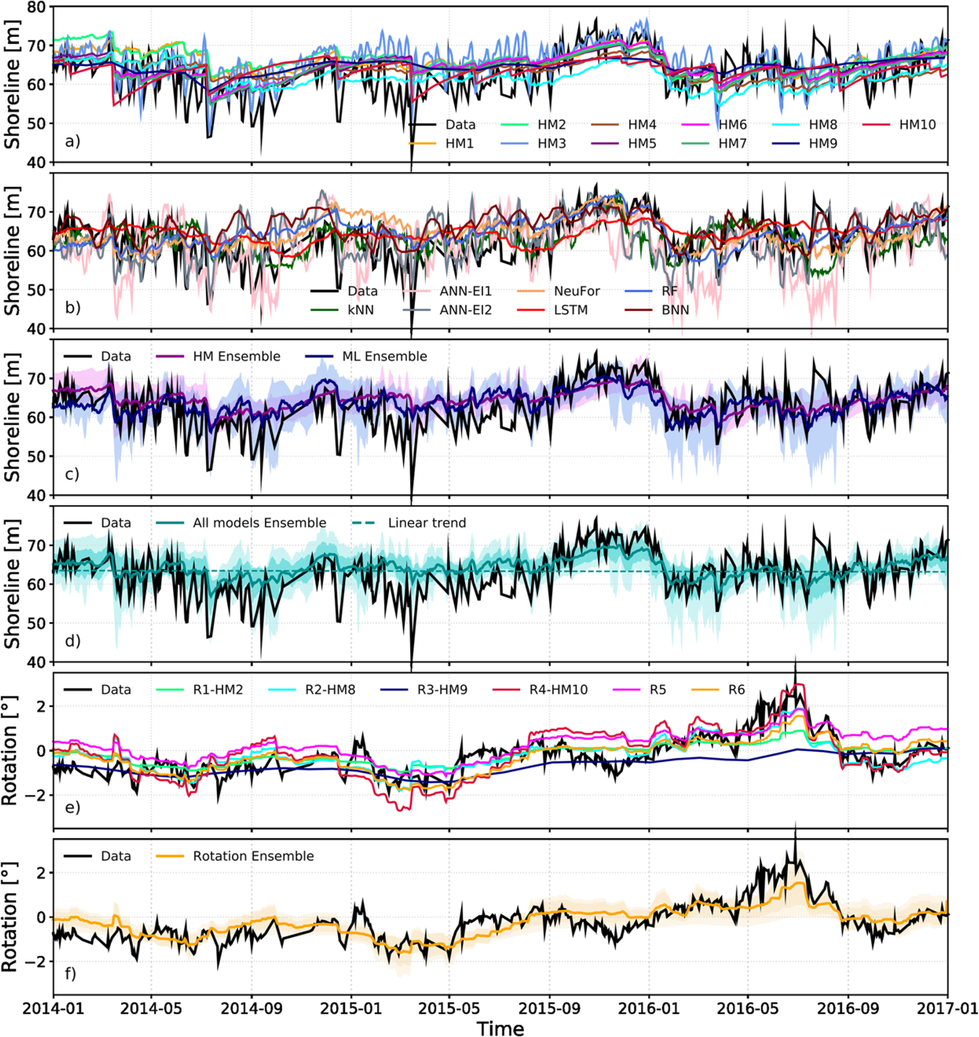
Monta├▒o et al. (2020) conducted a workshop and contest related to the shoreline fluctuation model ŌĆ£Shoreshop,ŌĆØ where participants from 15 international organizations tested and improved the performance of the model for predicting shoreline changes. They presented the result of a modeling contest, in which 19 models including the conventional numerical model were tested using the data pertaining to the daily average shoreline position and beach rotation for approximately 18 years (between 1999 and 2017) in the target sea, Tairua Beach. The result showed that the performance of the ML model was comparable to those of conventional numerical models. In fact, the multiyear variability at shorelines, which is difficult to simulate using conventional numerical models, can be analyzed easily using their model. Fig. 7 shows the results of shoreline fluctuations predicted using a numerical model, an ML model, and a hybrid model. Shoreline fluctuations during extreme events that occurred on a short time scale (Ōł╝monthly) was difficult to reproduce using the general numerical model. Meanwhile, the ML model adequately reproduced shoreline fluctuations in extreme events. However, the ability of the ML model in predicting the shoreline position deteriorated for the case involving data not used for training (2014ŌĆō2017). Therefore, the ML (inductive) and numerical (deductive) models complement each other in estimating shoreline fluctuations owing to their different approaches. Consequently, the ensemble approach combining the ML and numerical models improved the prediction reliability and reduced the uncertainty of the model.
4. Conclusions
In this study, we examined waves, tide level and sea level fluctuations, design variable estimation, and morphological changes in several studies that applied ML in coastal engineering. Based on extensive studies, the ML model proved to be a reliable in solving problems related to coastal engineering. The ML model can be constructed by learning the correlations between the input and output variables without basic mathematical and physical understanding pertaining to extremely complex interactions and processes associated with coastal engineering. However, several factors should be considered from the researcherŌĆÖs perspective to implement such highly accurate models, including the following:
-
Amount of data
A significant amount of training data with various ranges is required to construct an ML model. However, the exact amount of data required to derive meaningful prediction results remains elusive. Goldstein et al. (2019) reported that the performance deteriorates when a significant amount of data is applied to a low-complexity model in certain cases. These results cannot be generalized to all cases. However, the amount of data required for optimal prediction using the empirical knowledge of researchers and the method for managing noise in the data must be analyzed quantitatively. -
Data preprocessing
Actual data were acquired from various sources and processes; hence, incomplete data, noise, and inconsistent data that reduce the quality of the dataset may be included in the acquired data. Researchers must perform appropriate data preprocessing to improve data quality to achieve high-performance models. During data preprocessing, the model data should be converted into data suitable for the model through data cleaning, which replaces missing values or removes noise data and outliers. Furthermore, data normalization should be performed to reduce dimension and noise by via feature scale matching. For example, Zanuttigh et al. (2016) introduced a weight factor to the preprocessing process for more than 17,000 data points obtained from the CLASH database and reduced the data impurity via bootstrap sampling. Furthermore, the range of the dependent variables was 10ŌłÆ9< q < 10 but might be underestimated due to error calculation. Thus, a study was performed to improve the accuracy of the model by converting the dependent variable into log(q). The reliability and accuracy of the model could be further improved through appropriate data preprocessing based on the results of previous studies. -
Model analysis
An ML model is a black box model with a complex structure. Therefore, its intuitive interpretation ability is low for supporting the prediction results. To improve the limitations of such black box models, explainable artificial intelligence (XAI) is currently being conducted. The XAI methodology provides interpretation such that humans can understand the results predicted by ML algorithms. The model is reliable if the basis on which the model derived the prediction results through XAI can be determined. Furthermore, one can determine whether the model has been appropriately trained or whether the data used for training are appropriate. Kim et al. (2021) analyzed a wave transmission coefficient prediction model for low-crested structures using the Shapley additive explanation (SHAP). Simple ML models should be constructed and reliable model analyses should be conducted based on previous results. -
Model validation and generalization
ML models generally segregate the data into training and test datasets randomly. However, data under extreme conditions or data with important information may be excluded from the training process, and this possibility should be considered when segregating the data. The reliability of the model should be improved through cross-validation, such as the k-fold cross validation and leave one out cross-validation. Furthermore, the model constructed through verification should perform a generalization process using new data that have not been used for training. Monta├▒o et al. (2020) presented the results of blinding tests on a numerical model and an ML model through workshops and competitions pertaining to ŌĆ£Shoreshop,ŌĆØ which is a shoreline fluctuation model. The exchange and dissemination of knowledge among researchers worldwide should be promoted, and problems in coastal engineering should be solved from various angles through such modeling contests.
Coastal engineering researchers can obtain new knowledge and insights regarding data analysis via ML models. However, the ML model is an inductive approach rather than a deductive approach, which is the conventional approach used in numerical models. Hence, it is difficult to generalize the model based on the range and characteristics of the data. For example, in regard to the prediction of morphological changes, generalizing all regions based on a single model is difficult because the data characteristics of a specific region are reflected in the model. Therefore, various problems in the coastal engineering field should be solved using an ensemble model that combines the conventional numerical model with an ML model, and by deriving results that improve prediction performance through a mutual complement of their strengths and weaknesses.