


1. Introduction
Underwater acoustics is the study of all phenomena related to the occurrence, propagation, and reception of sound waves in the water medium. Because electromagnetic waves undergo a significant attenuation in water, sound waves, which have relatively low propagation loss and high propagation speed, are used for underwater communication and detection. In the field of underwater acoustics, studies are mainly conducted on underwater communications, underwater target detection, marine resources, and measurement and analysis of underwater sound sources.
Most applications for underwater acoustics can be described as remote sensing. Remote sensing is employed when an object, condition, or phenomenon of interest cannot be directly observed and information about the target of interest is acquired indirectly using data. In underwater acoustics, this can be described simply as a sound navigation and ranging (sonar) system. Sonar systems can be broadly classified into passive and active systems. Passive sonar systems acquire information by using sensors to measure the acoustic energy (signal) emitted by the target of interest. In active sonar systems, the observer obtains information by directly emitting an acoustic pulse and gathering the returning signals that are reflected by the target.
Machine learning, which is widely known today, was initially used in academia for developing artificial intelligence. Recently, the use of machine learning has become widespread owing to the introduction of high-speed parallel computing that uses graphics processing units (GPUs) and can perform reliable learning based on big data, as well as develop various machine learning techniques that can find optimal solutions. Machine learning has contributed to the evolution of acoustic signal processing and voice recognition, and it is also utilized in various ways in the field of underwater acoustics. It is used for traditional remote sensing, such as in detection/classification of underwater sound sources and targets and localization. In addition, it is being used in the field of acoustic signal processing for seabed classification and marine environment information extraction and is producing an abundance of scientific results.
Data-driven machine learning divides the data into a training set and test set. The training set is used to create a model that is suitable for machine learning, and the model’s accuracy is increased through a repetitive model update process in which the model is validated via the test set (Bishop, 2006; Murphy, 2012). Here, it is necessary to have a process for extracting features from the training set. Some existing machine learning algorithms require these features to be found through human intervention. However, if deep learning is used, this feature extraction process can be performed automatically, and the model’s accuracy can be improved markedly at the same time (Goodfellow et al., 2016). To use deep learning, big data is required, and the existing machine learning methods may be more appropriate than deep learning when a small number of computations are required in situations where there is insufficient data. Therefore, it can be said that there is a complementary relationship between deep learning and machine learning.
Many recent attempts have been made to apply various machine learning techniques, such as deep learning, to each aspect of underwater acoustics. However, due to the nature of the underwater environments, the use of these aggressive and open techniques is challenging because the data acquisition/processing procedure is more constrained than that on land (in the air). Therefore, in the field of underwater acoustics, there is a movement towards combining traditional underwater acoustic research techniques with machine learning and developing them in concert with each other.
This paper aims to understand how machine learning is applied to each aspect of underwater acoustics. The next section discusses the theories regarding the definitions, types, and basic concepts of machine learning.
2. Machine Learning Theory
2.1 Definitions, Types, and Basic Concepts of Machine Learning
Machine learning is a technology in which a machine (computer) uses data to automatically detect and even predict hidden characteristics or patterns (Bishop, 2006; Murphy, 2012). Therefore, machine learning can be regarded as data-driven, and the system performance is determined by the quality of the data. As such, it is very important to build databases that are quantitatively and qualitatively excellent. Machine learning methods can be generally classified into supervised and unsupervised learning. Supervised learning refers to learning the following mapping from N number of training data input/output pairs
{ ( x i , y i ) } i = 1 N
Here, x is the training data input and is referred to as a feature. It can have a complex structure such as an image or a time-series signal. In principle, the output y can be anything, but generally in the case of categorical variables, the problem in Eq. (1) becomes a problem of classification or pattern recognition. When y is a real value, it results in a regression problem (Bishop, 2006; Murphy, 2012). The most basic data set for creating such a system is called a sample. Normally, the collected samples are divided into two sets: a training set that is used to create the system and a test set that is used to evaluate the system’s performance after it has been created. The difference between f(x) which is predicted from the input x, and y which is actually obtained, is expressed as ϵ. In acoustics, this normally corresponds to noise.
In the second type of machine learning that is unsupervised learning, only the input x is provided without any sample class information, and the goal is to find new patterns in this input data. As such, it is a much less clear problem than supervised learning, and there is no clear error metric. In underwater acoustics, a considerable number of previous sonar application studies have used machine learning for classification purposes, such as target type/state classification (Choi et al., 2019; Fischell and Schmidt, 2015; Ke et al., 2018; Wang et al., 2019) and target and clutter signal classification (Allen et al., 2011; Murphy and Hines, 2014; Young and Hines, 2007). In many of these studies, the properties of the data that were used for learning were recognized beforehand owing to the goals of the studies. As such, supervised learning was mainly used rather than unsupervised learning. Besides, studies on underwater source localization (Das, 2017; Das and Sejnowski, 2017; Gemba et al., 2019; Gerstoft et al., 2016; Nannuru et al., 2019) or seabed classification (Buscombe and Grams, 2018; Diesing et al., 2014) have used various machine learning algorithms that include unsupervised learning.
In the aforementioned studies, the system input was also referred to as features. When performing learning, such as pattern recognition or classification, it is necessary to extract the features that will be used to classify samples. Features are more useful for classification when N number of classes have different values from each other; therefore, these can be considered good features. Observed samples are generally expressed in the form of feature vectors. However, because using many features is not necessarily favorable, it is important to select only the part of the feature set that is highly useful. In addition, the amount of computation may increase exponentially as the dimensions of the feature vectors increase. This is called the curse of dimensionality (Hastie et al., 2009; Murphy, 2012). As a result, feature extraction methods may vary according to the field where pattern recognition is used, and researchers often use methods that reduce dimensionality by converting the extracted feature values into different values or employing techniques such as principal component analysis (PCA) (Murphy, 2012).
There may be a vast variety of models in which a certain entered input is classified into one out of N number of classes. Sometimes, when there are models with various degrees of complexity, each model’s misclassification rate for the training set is calculated and compared to the others in order to select the most appropriate model (Hastie et al., 2009). However, machine learning systems are created to build models that recognize and classify new samples. Therefore, a true performance evaluation can only be accomplished by measuring the performance of the system using a sample set other than the training set, i.e., a test set. The performance that the system shows in regard to the test set is called generalization ability (Hastie et al., 2009). The standard for selecting machine learning models is to select models with excellent generalization ability. However, it may not be possible to use a test set depending on the circumstances. In such cases, the training set may be split in two, with one part used for training and other part used for measuring the model’s performance, assuming that the training set is very large. The latter sample set is called the validation set. In this case, the learning and validation process are repeated for several models, and the best model is selected (Hastie et al., 2009). In reality, there are many cases where there is insufficient data to split the training set in two. In such cases, researchers use resampling techniques that use the same sample several times. Typical methods include cross-validation and bootstrapping (Kohavi, 1995).
When we “recognize” events or objects, we usually calculate a “possibility” and recognize things as being “most likely.” This is a universal decision-making method, and machine learning systems also follow this principle. Samples that are observed from input patterns are expressed in the form of feature vector x, and this must be classified as the most likely class. Here, the qualitative standard of “most likely” is defined as the quantitative standard of the posterior probability p(y|x). That is, in classification problems, success is achieved by finding the class with the greatest posterior probability and classifying the target as that class. If it is based on Bayesian statistics, p(y|x) can be estimated by using the Bayes rule shown below (Bishop, 2006).
That is, it can be replaced by the product of prior probability p(y) and likelihood p(x|y). The probability distributions of each of these is estimated through learning or training, and the estimation methods can be broadly divided into parametric and nonparametric methods (Murphy, 2012). Parametric methods can only be applied to certain types of probability distributions that can be expressed as parameters. Typical methods include the maximum likelihood method and the maximum posterior method. The nonparametric method is suitable for cases that do not actually follow a certain probability distribution, and a well-known typical method is the k-nearest neighbor method.
In many cases, the process of estimating probability distributions is ultimately an optimization problem. The most important part of formulating a given problem as an optimization problem is defining the cost function. The cost function includes parameters, and the parameters that minimize or maximize the cost function are found. The process of finding the optimal solution depends greatly on differentiation and gradient-based algorithms, but other optimization algorithms can also be used (Goodfellow et al., 2016).
2.2 Supervised Learning
As mentioned previously, supervised learning can be divided into classification and regression. Classification can be categorized according to the number of output classes, from the simplest binary classification to multiclass classification. Regression is about estimating a certain continuous variable as the output.
2.2.1 Support vector machine (SVM)
An SVM is basically an algorithm that learns rules for data classification and regression. SVM is a method of creating a non-stochastic linear classification model that determines which class the data belongs to (for example, determining which group the data belongs to, out of two groups), assuming that the given data is in an n-dimensional vector space. A model that is created in this way can determine which class the newly entered data belongs to. Classification is generally directed toward maximizing the margin, which is defined as the minimum distance between the decision boundary and data of each class (Murphy, 2012).
The most basic goal of an SVM is to create the most complete linear classification model that classifies data into two groups (Fig. 1(a)). Such a classification model can generally be found by solving quadratic optimization problems. SVMs can be used even in cases where it is difficult to classify data with a linear model (Fig. 1(b)). To do this, the kernel trick is often used, as it transforms the dimensions of the training data and uses an SVM in a new space (Bishop, 2006).
2.2.2 Neural network: multi-layer perceptron
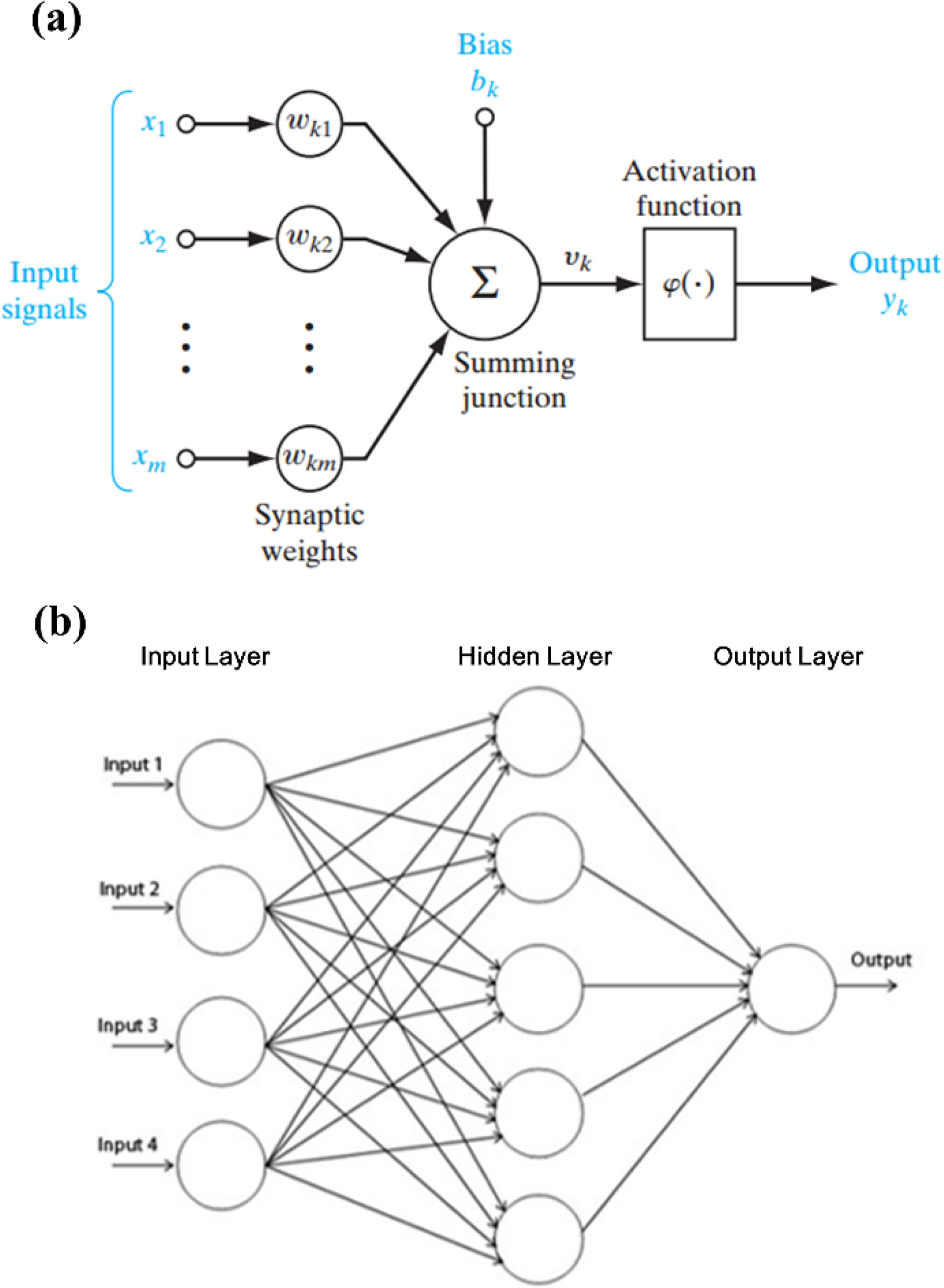
Deep neural networks are modeled after biological neural networks, and they have become widely known owing to deep learning. The neural networks that are described in this section are the initial form of the basic algorithm that was the precursor of deep neural networks. Neural networks are computation models in which there are many connections between numerous operators that perform simple calculations. The information processing procedure can be represented simply by y = f(x). The perceptron theory is an algorithm that can mathematically solve neural networks. The simplest perceptron model is a single-layer perceptron that consists of an input layer and output layer, as shown in Fig. 2(a) (Goodfellow et al., 2016).
In Fig. 2(a), the xi value is the input value, and wi is the weight for that value. The circle between the input layer and output layer is the activation function. The activation function makes the learning calculations easy by imitating a biological neuron that only allows signals to pass through if they are above a fixed level (Goodfellow et al., 2016). Single-layer perceptron can only be applied to problems that can be expressed linearly, and it is difficult to apply them to problems that have a nonlinear structure. This is resolved by adding new layers between the input layer and output layer. A neural network structure that includes a new layer between the input layer and output layer, i.e., a hidden layer, as shown in Fig. 2(b), is called a multi-layer perceptron. A neural network that has several hidden layers is called a deep neural network (Goodfellow et al., 2016). Deep neural networks are discussed again in the deep learning part of Section 2.4.
Each layer linearly combines the data inputted from the previous layer while considering the weights. The activation function is applied to these values, and they are sent to the next hidden layer. During this process, the activation function that is used for the hidden layer employs a threshold value to filter out insignificant values. Functions that allow for easy first-order differentiation (e.g., a sigmoid function) are often used to facilitate calculations. The number of hidden layers is solely determined by the intuition and experience of the designer (Goodfellow et al., 2016). However, it is necessary to consider the possibility of overfitting and the problem of computational complexity unavoidably increasing as the number of hidden layers increases. However, to properly design a neural network, it is also necessary to consider the problem of reduced calculation accuracy that can occur when there are too few hidden layers. The process of finding the optimal value for the weights in each layer is called learning.
2.3 Unsupervised Learning
The goal of unsupervised learning is to find an interesting structure that can properly describe new patterns or data from input data x without the sample’s class information. In sonar application research, various techniques that employ unsupervised learning have been attempted in studies on underwater source localization and seabed classification.
2.3.1 K-means clustering
K-means clustering is a simple unsupervised learning algorithm that performs clustering without the sample’s class information (MacQueen, 1967). K-means clustering assumes that the sample can be divided into k number of clusters and classifies the training data into the most appropriate clusters. This process is generally performed by considering the distance-based similarity between groups or minimizing the cost. Each data item is classified into the most appropriate cluster as the total cost or the sum of the total distance between the data and clusters is steadily reduced.
2.3.2 Principle component analysis
In PCA, the training set is used to estimate the parameters that are needed for data transformation, and these results are used to transform the feature space. That is, PCA transforms the raw signal into a lower-dimension feature vector. To perform the transformation, the high-dimension data’s variance is preserved as much as possible while finding a new low-dimension basis that is orthogonal and not linearly related (Murphy, 2012). The feature’s principal component can be obtained from the eigenvector of the covariance matrix Σ of the data.
Here, A = [a1 … aN] ∈ RN×N is the principal component vector, and
∑ 2 = diag ( [ σ 1 2 , ⋯ , σ N 2 ] ) ∈ R N × N
2.3.3 Gaussian mixture model
As stated in the name, a Gaussian mixture model (GMM) is a clustering model that combines several Gaussian distributions. Complex forms of probability distributions that actually exist are depicted by combining the K number of Gaussian distributions (McLachlan et al., 2019). In a GMM, for a given data item x, the probability that x will occur is expressed as the sum of several Gaussian probability density functions, as shown below.
Here, the mixture coefficient πk shows the probability of selecting the k-th Gaussian distribution. It is set so that 0 < πk ≤ 1 and
∑ k = 1 K π k = 1
2.3.4 Autoencoder
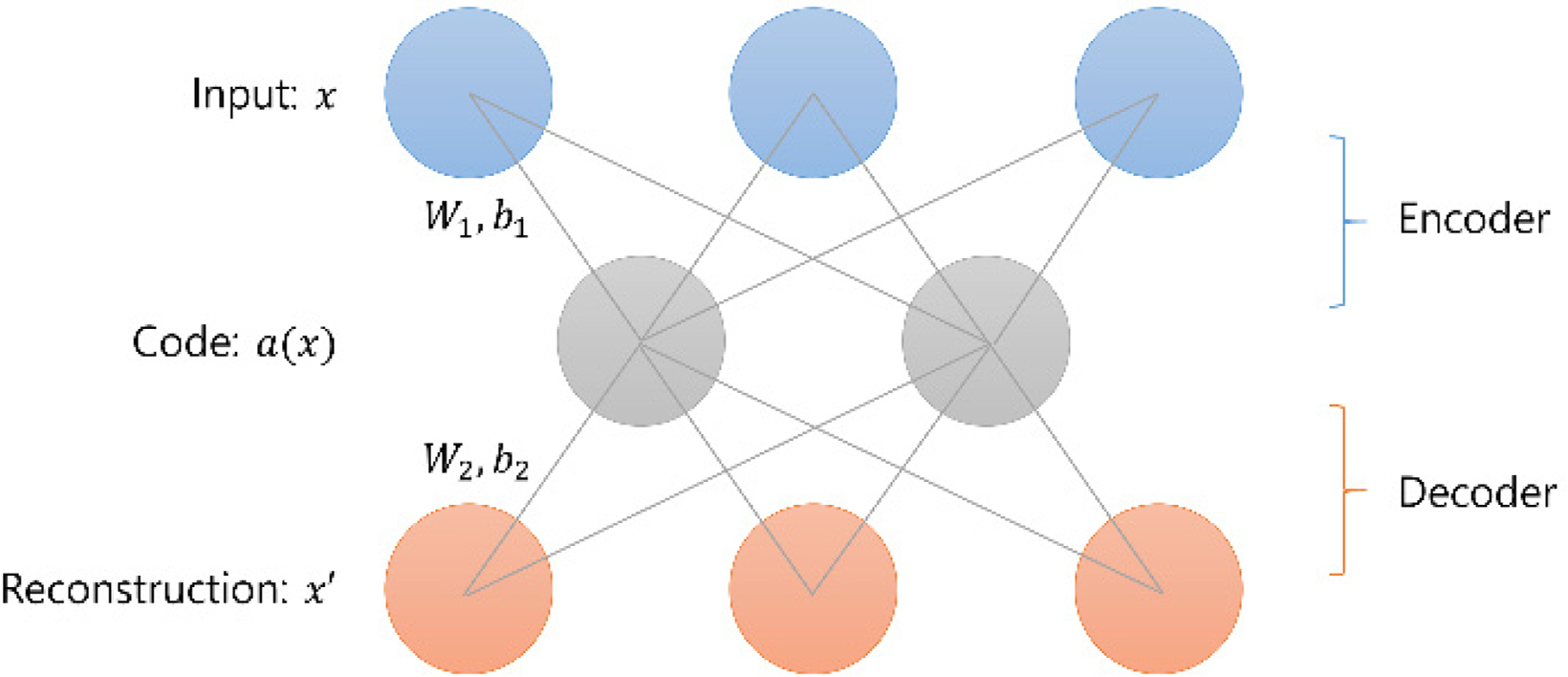
An autoencoder is a type of unsupervised neural network, and it is often used to reduce dimensions or search feature spaces. In simple terms, an autoencoder is a neural network that copies the input values to the output values, but it has evolved in various ways via methods that apply several types of regularization to the neural network according to its purpose (Goodfellow et al., 2016). For example, as shown in Fig. 3, various autoencoders can be created, such as autoencoders that compress data by making the number of hidden layer neurons smaller than the input layer or autoencoders that train neural networks so that they can restore the original input after noise is added to the input data. This regularization prevents the unsupervised neural network from simply copying the input directly to the output, and it is adjusted to learn methods of efficiently representing data.
2.3.5 Sparse dictionary learning
Researchers have developed and applied various types of methods for introducing sparse coding to reduce the dimensions of the data that is to be processed (Elad, 2010). One of these, sparse dictionary learning, has the goal of finding sparse representations of input data in the form of the input data’s basic elements or linear combinations of basic elements (Elad, 2010; Tosic and Frossard, 2011). For example, in x = Dα, x is the input data, and D is defined as the dictionary matrix. Here, the elements of D are defined as atoms. That is, x can be expressed as a linear combination of the column vector atoms that make up the dictionary. The solution that has the most coefficients that are 0 is found from among α. This is expressed mathematically, as shown below.
α* is the sparse representation coefficient. The constraint condition ‖∙‖0 represents the l0-norm. This is a method of finding the total number of elements that are not 0 in the vector. However, the l0-norm is a non-convex function, and thus, it has difficulty finding an accurate solution. As an alternative, it is sometimes changed to the l1-norm constraint condition, and a fast approximate solution method such as orthogonal matching pursuit (Elad, 2010) or sparse Bayesian learning (Wipf and Rao, 2004) is used.
2.4 Deep learning
As implied by the name, today’s deep learning methods are learning techniques that employ deep neural networks (Goodfellow et al., 2016). Previously, it was mentioned that a deep neural network is a complex neural network structure that includes several hidden layers and is based on a multi-layer perceptron structure. As such, it can be considered a machine learning model with a high level of complexity, and this is a structure that is similar to the series of neural layers that gradually extract complex information in the human brain. That is, relatively simple information processing is performed in the lower layers, and more complex information is extracted at the higher layers.
In deep neural networks, learning is performed by optimizing the weights in each layer. The main method for deep neural network learning is the backpropagation algorithm (Rumelhart et al., 1986). This approach mainly uses the gradient descent method to continually propagate the error in the back direction to obtain the optimal weights. The backpropagation method shows very good performance for simple problems, but as the neural network’s structure becomes more complex, several serious weaknesses become apparent. First, as the neural network’s structure becomes more complex, the number of weights increases, and a large amount of learning data is required. In addition, the number of hidden layers increases, and the strength of the error weakens as it is backpropagated from the output layer to the input layer, making it difficult to perform learning. Because of these limitations, research on deep neural networks was stagnant for some time. Later, a considerable number of the aforementioned problems were resolved by using methods such as preprocessing each layer of the neural network using an unsupervised learning technique such as a restricted Boltzmann machine (RBM), using a rectified linear unit (ReLU) function as a new activation function, and preventing overfitting by including a regularization step in the learning process (Goodfellow et al., 2016). In addition to these technological advances, the construction of systems that can easily acquire large amounts of data, as well as huge advances in the computing capacity of GPUs, have allowed current learning techniques that use deep neural networks to provide performance that is vastly superior to the conventional machine learning techniques.
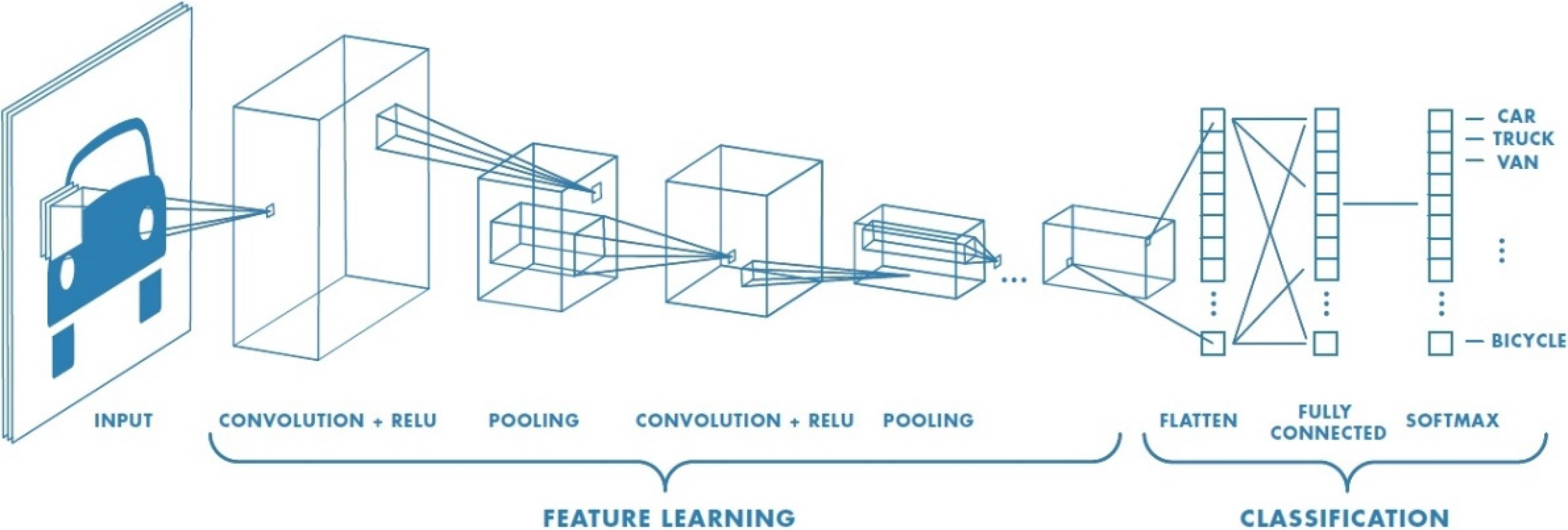
Currently, most deep learning models are based on convolutional neural networks (CNN). A CNN (Fukushima, 1980; LeCun et al., 1998) is a deep neural network that imitates the human visual recognition process, and it can be considered a neural network that is optimized for the field of image recognition. CNNs support convolution, and because of this characteristic, they are more useful than normal neural networks for receiving and learning input data of two dimensions or more. They have the advantage of being able to learn high-dimension data with relatively few parameters. Normally, CNNs consist of convolutional layers and pooling layers that extract the features of high-dimension data, as well as a fully connected layer that ultimately classifies the data. The order and number of the convolutional and pooling layers can be adjusted as needed according to the problem that the user is solving.
Convolution is used to separate and extract the features of input data, such as images. Specialized filters are used to extract features that consist of certain colors or tones in an image, and these filters and the input data can be convoluted to extract emphasized image features according to the characteristics of each filter. If this is repeated several times, ultimately the CNN can recognize the image. Due to these structural features, for higher-dimension analysis problems using images, CNNs show unrivaled performance compared to other algorithms. In the field of underwater acoustics, CNNs are actively being used to solve recognition and classification problems by transforming the input data into a frequency-time domain image using a short-time Fourier transform or a wavelet transform, depicting the input data in the range-azimuth domain, or using array signal processing.
3. Conclusions
In this paper, a brief discussion of the theory of machine learning, including deep learning is provided from a general perspective before examining the research trends in underwater acoustics using machine learning. This paper outlines the definitions, types, and basic concepts of machine learning and introduces the main techniques that are used in underwater acoustics and sonar applications, which will be discussed in earnest in a follow-up paper. The follow-up paper will provide a more detailed discussion of how machine learning is used in the main fields of interest in underwater acoustics, including underwater sound source and target detection/classification, localization, and ocean information extraction.
The process of data-driven machine learning includes establishing a model that is suitable for its purpose, performing training and validation via datasets, and improving accuracy by performing repeated model updates. Considering that the measurement environment and measurement data quality in each research field are completely different, it would be best to use machine learning in concert with conventional methods in accordance with the goals of the research. Owing to the nature of underwater environments, there are some challenges in using more aggressive and open techniques because the data acquisition/processing procedure is more constrained than that used on land (in the air). Therefore, there is a movement towards combining traditional research techniques and machine learning techniques and developing them in concert with each other. The follow-up to this paper will provide a detailed examination of the research flow for underwater acoustics and sonar signal processing that directly employs machine learning.